Finite-size scaling: extracting critical exponents

A single finite lattice can only show a rounded phase transition – true singularities require an infinite system. Finite-size scaling theory turns this apparent limitation into a tool: by simulating several lattice sizes and comparing how observables scale with \(L\), the exponents of the infinite system can be extracted without ever simulating one.

This example works with the 2D Ising ferromagnet, \(H = -J \sum_{\langle i,j \rangle} s_i s_j\) with \(s_i = \pm 1\) on a periodic \(L \times L\) lattice, and sweeps several lattice sizes across its exact critical temperature \(T_C\), estimating \(\gamma/\nu\) (from the scaling of the susceptibility peak), \(\beta/\nu\) (from the order parameter at \(T_C\)), and \(\nu\) (from the Binder cumulant’s slope at \(T_C\)) – comparing against the exact 2D Ising values \(\gamma=7/4\), \(\beta=1/8\), \(\nu=1\).

import matplotlib.pyplot as plt
import numpy as np

from physicskit.statphys.chapters.ising_lattice import Ising2D
from physicskit.statphys.utils.finite_size_scaling import (
    binder_cumulant_crossing,
    estimate_beta_over_nu,
    estimate_gamma_over_nu,
    estimate_nu_from_binder_slope,
)
from physicskit.statphys.utils.thermodynamics import binder_cumulant, susceptibility

Sweep several lattice sizes across T_C

L_values = [8, 16, 24, 32]
T_c_exact = Ising2D().T_C
temperatures = np.linspace(T_c_exact - 0.6, T_c_exact + 0.6, 21)

chi_max, m_at_tc, T_grids, U4_grids, chi_grids, M_grids = [], [], [], [], [], []

for L in L_values:
    model = Ising2D(L=L, seed=0)
    U4 = np.empty(len(temperatures))
    chi = np.empty(len(temperatures))
    M_mean = np.empty(len(temperatures))

    for k, T in enumerate(temperatures):
        beta = 1.0 / T
        model.sweep(beta, algorithm="wolff", n_sweeps=150)  # equilibrate
        mags = np.empty(500)
        for m in range(500):
            model.sweep(beta, algorithm="wolff", n_sweeps=1)
            mags[m] = model.magnetization()
        U4[k] = binder_cumulant(mags)
        chi[k] = susceptibility(np.abs(mags), T, model.n_sites)
        M_mean[k] = np.abs(mags).mean() / model.n_sites

    chi_max.append(chi.max())
    idx_tc = np.argmin(np.abs(temperatures - T_c_exact))
    m_at_tc.append(M_mean[idx_tc])
    T_grids.append(temperatures)
    U4_grids.append(U4)
    chi_grids.append(chi)
    M_grids.append(M_mean)

Extract the critical exponents

gamma_over_nu = estimate_gamma_over_nu(L_values, chi_max)
beta_over_nu = estimate_beta_over_nu(L_values, m_at_tc)
nu = estimate_nu_from_binder_slope(L_values, T_grids, U4_grids, T_c_exact)
T_c_fss = binder_cumulant_crossing(temperatures, dict(zip(L_values, U4_grids)))

The raw sweeps: sharpening signatures with growing L

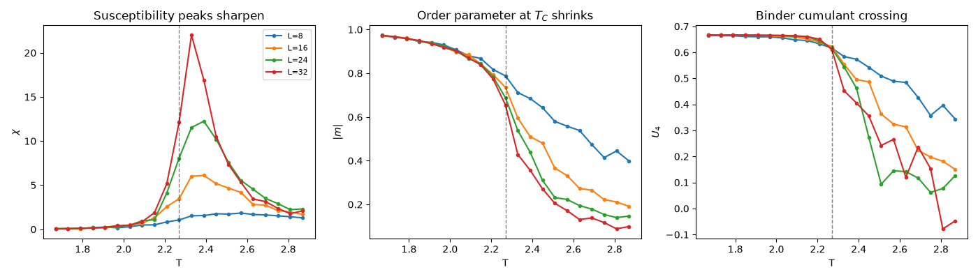
Susceptibility peaks grow and narrow with L (diverging as L^{gamma/nu} in the infinite-volume limit), the order parameter at T_C shrinks toward zero as L^{-beta/nu}, and the Binder cumulant curves for different L all cross at (approximately) the same T_C – the standard qualitative signatures that motivate the exponent extraction below.

fig, axes = plt.subplots(1, 3, figsize=(14, 4))
for L, T, chi, M, U4 in zip(L_values, T_grids, chi_grids, M_grids, U4_grids):
    axes[0].plot(T, chi, marker="o", ms=3, label=f"L={L}")
    axes[1].plot(T, M, marker="o", ms=3, label=f"L={L}")
    axes[2].plot(T, U4, marker="o", ms=3, label=f"L={L}")
for ax, ylabel, title in zip(
    axes,
    [r"$\chi$", r"$|m|$", r"$U_4$"],
    ["Susceptibility peaks sharpen", "Order parameter at $T_C$ shrinks", "Binder cumulant crossing"],
):
    ax.axvline(T_c_exact, color="k", linestyle="--", linewidth=1, alpha=0.5)
    ax.set_xlabel("T")
    ax.set_ylabel(ylabel)
    ax.set_title(title)
axes[0].legend(fontsize=8)
plt.tight_layout()

Finite-size scaling collapse

Rescaling each L’s curve by the fitted exponents – chi * L^{-gamma/nu} against (T - T_C) * L^{1/nu}, and |m| * L^{beta/nu} against the same rescaled temperature axis – should collapse all four lattice sizes onto a single universal curve near T_C if the fitted exponents are correct; how well the curves overlap is itself a visual check on the exponent fit.

fig, axes = plt.subplots(1, 2, figsize=(11, 4.5))
for L, T, chi, M in zip(L_values, T_grids, chi_grids, M_grids):
    x = (T - T_c_exact) * L ** (1.0 / nu)
    axes[0].plot(x, chi * L ** (-gamma_over_nu), marker="o", ms=3, label=f"L={L}")
    axes[1].plot(x, M * L ** (beta_over_nu), marker="o", ms=3, label=f"L={L}")
axes[0].set_xlabel(r"$(T - T_C)\, L^{1/\nu}$")
axes[0].set_ylabel(r"$\chi \, L^{-\gamma/\nu}$")
axes[0].set_title("Susceptibility collapse")
axes[0].legend(fontsize=8)
axes[1].set_xlabel(r"$(T - T_C)\, L^{1/\nu}$")
axes[1].set_ylabel(r"$|m|\, L^{\beta/\nu}$")
axes[1].set_title("Order parameter collapse")
plt.tight_layout()
plt.show()

print(f"gamma/nu = {gamma_over_nu:.3f}  (exact: 1.750)")
print(f"beta/nu  = {beta_over_nu:.3f}  (exact: 0.125)")
print(f"nu       = {nu:.3f}  (exact: 1.000)")
print(f"T_C (Binder crossing) = {T_c_fss:.3f}  (exact: {T_c_exact:.3f})")
print(
    "\nNote: gamma/nu, beta/nu, and T_C converge well even at these modest sizes and\n"
    "sample counts. nu is the hardest exponent to pin down this way -- it comes from\n"
    "a finite-difference derivative of an already-noisy quantity, and genuinely needs\n"
    "much larger L and far more samples per point to converge tightly; a visibly noisy\n"
    "estimate here is expected, not a bug."
)

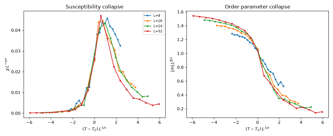
gamma/nu = 1.775  (exact: 1.750)
beta/nu  = 0.133  (exact: 0.125)
nu       = 1.512  (exact: 1.000)
T_C (Binder crossing) = 2.247  (exact: 2.269)

Note: gamma/nu, beta/nu, and T_C converge well even at these modest sizes and
sample counts. nu is the hardest exponent to pin down this way -- it comes from
a finite-difference derivative of an already-noisy quantity, and genuinely needs
much larger L and far more samples per point to converge tightly; a visibly noisy
estimate here is expected, not a bug.