Gibbs’s canonical ensemble: response from fluctuations

Gibbs (1902) described a system in contact with a heat bath not by one trajectory but by a probability distribution over all its states, \(p_s = e^{-\beta E_s}/Z\). Everything thermodynamic follows from the partition function \(Z=\sum_s e^{-\beta E_s}\). In particular, the heat capacity, which is a response to changing temperature, equals the size of the energy’s equilibrium fluctuations:

\[C = \frac{\partial\langle E\rangle}{\partial T} = \frac{\langle E^2\rangle - \langle E\rangle^2}{k_BT^2}.\]

A 4x4 periodic Ising lattice has only \(2^{16}=65{,}536\) states, so the canonical ensemble can be summed exactly. This example checks Gibbs’s identity term by term, then shows that the fluctuation formulas in specific_heat() and susceptibility(), applied to Monte Carlo samples from Ising2D, recover the exact ensemble values.

import matplotlib.pyplot as plt
import numpy as np

from physicskit.statphys.chapters.ising_lattice import Ising2D
from physicskit.statphys.utils.thermodynamics import specific_heat, susceptibility

L, J = 4, 1.0
N = L * L

Enumerate every state

states = ((np.arange(2**N)[:, None] >> np.arange(N)) & 1) * 2 - 1
spins = states.reshape(-1, L, L)
E = -J * (np.sum(spins * np.roll(spins, 1, axis=1), axis=(1, 2)) + np.sum(spins * np.roll(spins, 1, axis=2), axis=(1, 2)))
M = spins.sum(axis=(1, 2))
E_levels, g = np.unique(E, return_counts=True)
print(f"{2**N} states in {len(E_levels)} energy levels; ground-state degeneracy {g[0]}")


def ensemble(T):
    w = np.exp(-(E - E.min()) / T)
    Z = w.sum()
    avg = lambda q: np.sum(q * w) / Z  # noqa: E731
    return avg(E), avg(E**2), avg(np.abs(M)), avg(M**2)


T = np.linspace(0.8, 5.0, 200)
E_mean = np.array([ensemble(t)[0] for t in T])
C_fluct = np.array([(ensemble(t)[1] - ensemble(t)[0] ** 2) / t**2 for t in T]) / N
C_deriv = np.gradient(E_mean, T) / N
print(f"max |C_fluctuation - dE/dT| per site: {np.max(np.abs(C_fluct - C_deriv)[2:-2]):.1e}  (finite-difference error)")

65536 states in 15 energy levels; ground-state degeneracy 2
max |C_fluctuation - dE/dT| per site: 1.8e-04  (finite-difference error)

Monte Carlo samples recover the ensemble

Metropolis sampling visits states with Gibbs’s probabilities, so the variance of the sampled energy and magnetization gives \(C\) and \(\chi\) directly.

T_mc = np.array([1.5, 2.0, 2.5, 3.0, 4.0])
C_mc, chi_mc, chi_exact = [], [], []
for t in T_mc:
    model = Ising2D(L=L, J=J, seed=1902)
    model.sweep(1 / t, n_sweeps=2000)
    Es, Ms = [], []
    for _ in range(40000):
        model.sweep(1 / t)
        Es.append(model.energy())
        Ms.append(abs(model.magnetization()))
    C_mc.append(specific_heat(np.array(Es), t, N))
    chi_mc.append(susceptibility(np.array(Ms), t, N))
    _, _, Mabs, M2 = ensemble(t)
    chi_exact.append((M2 - Mabs**2) / (t * N))
    print(f"T = {t}: C/N  MC {C_mc[-1]:.4f}  exact {np.interp(t, T, C_fluct):.4f};   chi  MC {chi_mc[-1]:.4f}  exact {chi_exact[-1]:.4f}")

fig, (ax1, ax2) = plt.subplots(1, 2, figsize=(11, 4))
ax1.plot(T, C_deriv, color="steelblue", lw=3, alpha=0.5, label=r"$\partial\langle E\rangle/\partial T$")
ax1.plot(T, C_fluct, "k--", label=r"$(\langle E^2\rangle-\langle E\rangle^2)/T^2$")
ax1.plot(T_mc, C_mc, "o", color="firebrick", label="Metropolis samples")
ax1.set_xlabel("temperature T")
ax1.set_ylabel("heat capacity per spin")
ax1.set_title("4x4 Ising: response = fluctuation")
ax1.legend(fontsize=8)
ax2.bar(
    E_levels,
    g * np.exp(-(E_levels - E_levels.min()) / 2.5) / np.sum(g * np.exp(-(E_levels - E_levels.min()) / 2.5)),
    width=3,
    color="steelblue",
    alpha=0.7,
    label="exact, T = 2.5",
)
model = Ising2D(L=L, J=J, seed=1)
model.sweep(1 / 2.5, n_sweeps=2000)
sampled = []
for _ in range(20000):
    model.sweep(1 / 2.5)
    sampled.append(model.energy())
vals, counts = np.unique(sampled, return_counts=True)
ax2.plot(vals, counts / counts.sum(), "o", color="firebrick", label="Metropolis")
ax2.set_xlabel("energy E")
ax2.set_ylabel("probability")
ax2.set_title(r"Energy distribution: $g(E)\,e^{-E/T}/Z$")
ax2.legend(fontsize=8)
fig.tight_layout()

plt.show()

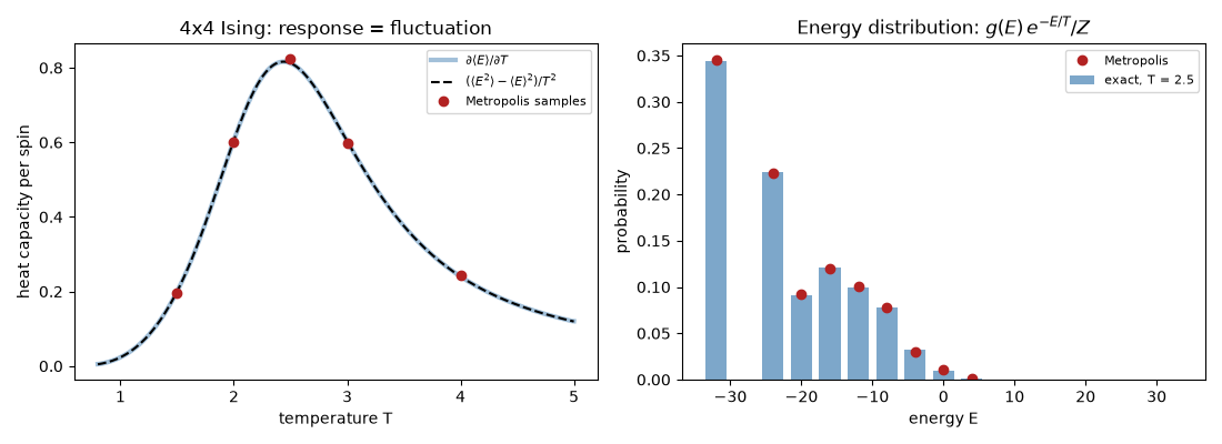
T = 1.5: C/N  MC 0.1945  exact 0.2004;   chi  MC 0.0273  exact 0.0295
T = 2.0: C/N  MC 0.5994  exact 0.6055;   chi  MC 0.1943  exact 0.1957
T = 2.5: C/N  MC 0.8237  exact 0.8124;   chi  MC 0.4529  exact 0.4483
T = 3.0: C/N  MC 0.5978  exact 0.6031;   chi  MC 0.4747  exact 0.4770
T = 4.0: C/N  MC 0.2421  exact 0.2401;   chi  MC 0.2944  exact 0.2934

Check

Exact enumeration: 2^16 states, a doubly degenerate ground state, and C = (<E^2> - <E>^2)/T^2 = d<E>/dT. Metropolis samples the same ensemble.

assert len(E) == 2**N and g[0] == 2
assert np.max(np.abs(C_fluct - C_deriv)[2:-2]) < 1e-3
C_exact = np.interp(T_mc, T, C_fluct)
assert np.max(np.abs(np.array(C_mc) / C_exact - 1)) < 0.05
assert np.max(np.abs(np.array(chi_mc) / np.array(chi_exact) - 1)) < 0.1
p_boltzmann = g * np.exp(-(E_levels - E_levels.min()) / 2.5)
p_boltzmann /= p_boltzmann.sum()
p_sampled = np.array([counts[vals == e].sum() for e in E_levels]) / counts.sum()
assert np.max(np.abs(p_sampled - p_boltzmann)) < 0.01