Watching criticality: the Ising lattice at T_C

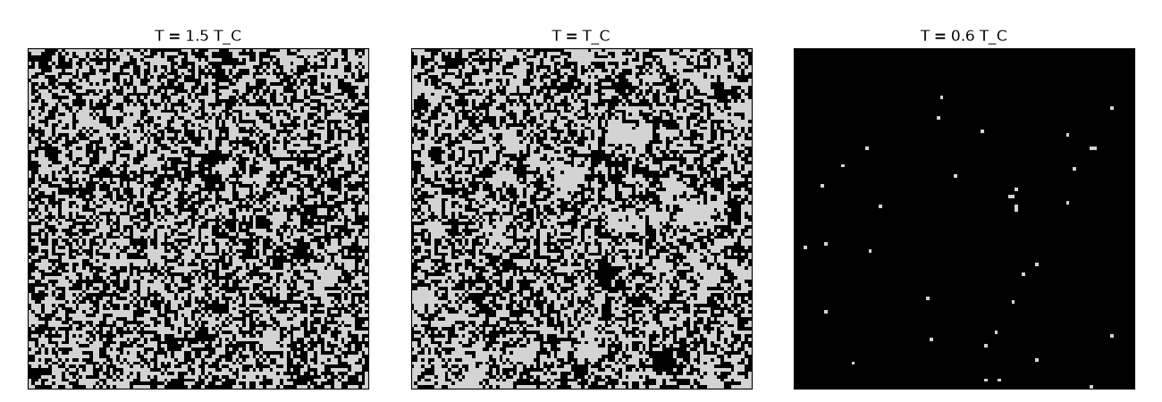
Away from \(T_C\), the 2D Ising lattice’s equilibrium configurations look qualitatively different above and below the transition: a fine, short-range-correlated speckle in the disordered phase, or a few large, slowly fluctuating domains in the ordered phase. Exactly at \(T_C\), neither picture applies – the correlation length

\[\xi(T) \sim |T - T_C|^{-\nu}, \qquad \nu = 1\]

diverges, so the lattice has no characteristic domain size at all: clusters of aligned spins appear at every scale simultaneously, from a handful of sites up to the size of the lattice itself, and that same scale-free structure keeps reappearing as the configuration evolves. Wolff’s cluster algorithm makes this directly visible frame by frame, since each move flips one such cluster – of whatever size the critical correlations happen to produce – as a single event.

import matplotlib.pyplot as plt
from matplotlib.colors import ListedColormap

from physicskit.statphys.chapters.ising_lattice import Ising2D
from physicskit.statphys.visualizers.lattice_render import animate_lattice_sweeps, plot_spin_grid

# Two-valued spin configurations (s = +-1) render more clearly as light grey
# vs. black than the default blue/red "coolwarm" colormap.
SPIN_CMAP = ListedColormap(["black", "lightgrey"])

Off-critical vs. critical snapshots

Equilibrated snapshots well above, well below, and exactly at T_C show the qualitative difference directly: fine disordered speckle, large ordered domains, and – at T_C itself – structure at every scale in between.

L = 100
fig, axes = plt.subplots(1, 3, figsize=(13, 4.5))
for ax, T_frac, label in zip(axes, [1.5, 1.0, 0.6], ["T = 1.5 T_C", "T = T_C", "T = 0.6 T_C"]):
    model = Ising2D(L=L, seed=0)
    T = T_frac * model.T_C
    model.sweep(1.0 / T, algorithm="wolff", n_sweeps=150)
    plot_spin_grid(model.spins, ax=ax, title=label, cmap=SPIN_CMAP)
plt.tight_layout()
plt.subplots_adjust(top=0.88)  # tight_layout alone leaves the titles clipped by the figure edge
plt.show()

Animation: Wolff clusters flipping at T_C

Each frame is a fixed number of Wolff cluster flips at beta = 1/T_C; watch clusters of every size, from a few sites to a large fraction of the lattice, appear and flip in turn – the direct, visual signature of a diverging correlation length, with no separate “measurement” required.

model = Ising2D(L=L, seed=1)
beta_c = 1.0 / model.T_C
model.sweep(beta_c, algorithm="wolff", n_sweeps=20)  # equilibrate at T_C first
anim = animate_lattice_sweeps(model, beta_c, n_frames=150, sweeps_per_frame=1, algorithm="wolff", cmap=SPIN_CMAP)
plt.show()

To save the animation to a file instead of (or in addition to) displaying it interactively, use e.g.:

anim.save("ising_criticality.gif", writer="pillow", fps=10)