Onsager’s exact solution: the 2D Ising phase transition

The 2D Ising model places a spin \(s_i = \pm 1\) on every site of a periodic \(L \times L\) lattice, with Hamiltonian

\[H = -J \sum_{\langle i,j \rangle} s_i s_j,\]

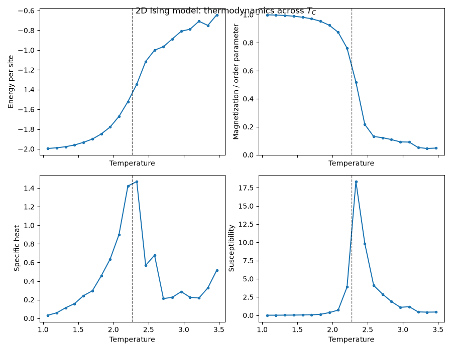
summed over nearest-neighbor pairs. It is the simplest system with a genuine continuous (second-order) phase transition, and the only nontrivial one solved exactly – by Lars Onsager in 1944. Below the critical temperature \(T_C = 2J / (k_B \ln(1+\sqrt{2})) \approx 2.269\, J/k_B\), the system spontaneously magnetizes; above it, thermal fluctuations destroy the order. This example sweeps temperature across \(T_C\) on an \(L=32\) lattice with the cluster-flipping Wolff algorithm (to avoid critical slowing down) and reproduces the textbook signatures of the transition: the magnetization order parameter dropping to zero, and the specific heat and susceptibility both peaking at \(T_C\).

import matplotlib.pyplot as plt
import numpy as np
from matplotlib.colors import ListedColormap

from physicskit.statphys.chapters.ising_lattice import Ising2D
from physicskit.statphys.visualizers.lattice_render import plot_spin_grid, plot_thermodynamics

# Two-valued spin configurations (s = +-1) render more clearly as light grey
# vs. black than the default blue/red "coolwarm" colormap.
SPIN_CMAP = ListedColormap(["black", "lightgrey"])

Sweep temperature across the transition

Sampling from high to low temperature lets each equilibration step start from the (already close to equilibrium) previous configuration.

model = Ising2D(L=32, J=1.0, kB=1.0, seed=0)
temperatures = np.linspace(model.T_C + 1.2, max(model.T_C - 1.2, 0.5), 20)
result = model.run_temperature_sweep(temperatures, n_equil=200, n_measure=300, algorithm="wolff")

plot_thermodynamics(result, T_c=model.T_C)
plt.suptitle("2D Ising model: thermodynamics across $T_C$")

Text(0.5, 0.98, '2D Ising model: thermodynamics across $T_C$')

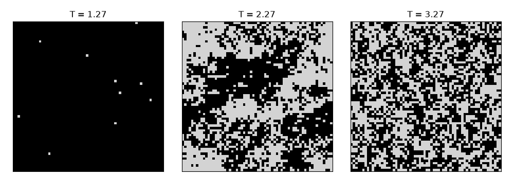
Snapshots below, at, and above \(T_C\)

fig, axes = plt.subplots(1, 3, figsize=(10, 3.5))
for ax, T in zip(axes, [model.T_C - 1.0, model.T_C, model.T_C + 1.0]):
    snapshot_model = Ising2D(L=64, J=1.0, kB=1.0, seed=1)
    snapshot_model.sweep(beta=1.0 / T, algorithm="wolff", n_sweeps=200)
    plot_spin_grid(snapshot_model.spins, ax=ax, title=f"T = {T:.2f}", cmap=SPIN_CMAP)
plt.tight_layout()
plt.subplots_adjust(top=0.88)  # tight_layout alone leaves the titles clipped by the figure edge
plt.show()