The Metropolis algorithm: sampling Boltzmann without the partition function

Metropolis, the Rosenbluths and the Tellers (1953) showed how to draw states with Boltzmann probability \(e^{-\beta E}/Z\) without ever computing \(Z\). Propose a small random change; accept it with probability \(\min(1, e^{-\beta\Delta E})\). The rule satisfies detailed balance, \(p_a P(a\to b) = p_b P(b\to a)\), so the chain’s stationary distribution is exactly Boltzmann’s, from any starting state.

A 3x3 periodic Ising lattice has 512 states, few enough to compute the exact distribution. This example checks the acceptance rule, runs metropolis_sweep_ising() (via Ising2D) from an ordered and a random start, and compares the sampled energy histogram with the exact one, at a temperature where direct sampling of random configurations would almost never hit the important states.

import matplotlib.pyplot as plt
import numpy as np

from physicskit.statphys.chapters.ising_lattice import Ising2D

L, J, T = 3, 1.0, 2.5
beta = 1.0 / T
N = L * L

Exact Boltzmann distribution

states = ((np.arange(2**N)[:, None] >> np.arange(N)) & 1) * 2 - 1
spins = states.reshape(-1, L, L)
E = -J * (np.sum(spins * np.roll(spins, 1, 1), axis=(1, 2)) + np.sum(spins * np.roll(spins, 1, 2), axis=(1, 2)))
levels, degeneracy = np.unique(E, return_counts=True)
p_exact = degeneracy * np.exp(-beta * (levels - levels.min()))
p_exact /= p_exact.sum()
print("E      g(E)   Boltzmann P(E)   uniform P(E)")
for e, gd, p in zip(levels, degeneracy, p_exact):
    print(f"{e:5.0f} {gd:6d}   {p:14.5f}   {gd / 2**N:12.5f}")

E      g(E)   Boltzmann P(E)   uniform P(E)
  -18      2          0.56932        0.00391
  -10     18          0.20886        0.03516
   -6     48          0.11245        0.09375
   -2    198          0.09365        0.38672
    2    144          0.01375        0.28125
    6    102          0.00197        0.19922

The acceptance rule and detailed balance

For a single spin flip in the Ising model, \(\Delta E\) can only be \(-8J,-4J,0,4J,8J\). Moves downhill are always taken; uphill moves only with the Boltzmann factor. The ratio of forward to backward acceptance equals the ratio of Boltzmann weights, which is detailed balance.

for dE in (-8, -4, 0, 4, 8):
    a_fwd, a_back = min(1, np.exp(-beta * dE)), min(1, np.exp(beta * dE))
    print(f"dE = {dE:+d}J: accept {a_fwd:.4f}, reverse {a_back:.4f}, ratio {a_fwd / a_back:.4f} = exp(-beta dE) {np.exp(-beta * dE):.4f}")

dE = -8J: accept 1.0000, reverse 0.0408, ratio 24.5325 = exp(-beta dE) 24.5325
dE = -4J: accept 1.0000, reverse 0.2019, ratio 4.9530 = exp(-beta dE) 4.9530
dE = +0J: accept 1.0000, reverse 1.0000, ratio 1.0000 = exp(-beta dE) 1.0000
dE = +4J: accept 0.2019, reverse 1.0000, ratio 0.2019 = exp(-beta dE) 0.2019
dE = +8J: accept 0.0408, reverse 1.0000, ratio 0.0408 = exp(-beta dE) 0.0408

Two starts, one distribution

From the all-up state and from a random state the running average of the energy converges to the same exact value, and the histogram of visited energies matches Boltzmann’s distribution.

E_exact = np.sum(levels * p_exact)
traces, hist = {}, {}
for label, ordered in (("ordered start", True), ("random start", False)):
    model = Ising2D(L=L, J=J, seed=1953 + ordered)
    model.reset(ordered=ordered)
    Es = []
    for _ in range(40000):
        model.sweep(beta)
        Es.append(model.energy())
    Es = np.array(Es)
    traces[label] = np.cumsum(Es) / np.arange(1, Es.size + 1)
    hist[label] = np.array([np.mean(Es[1000:] == e) for e in levels])
    print(f"{label}: <E> = {Es[1000:].mean():.4f}  (exact {E_exact:.4f})")

fig, (ax1, ax2) = plt.subplots(1, 2, figsize=(11, 4))
for label, tr in traces.items():
    ax1.semilogx(np.arange(1, tr.size + 1), tr, label=label)
ax1.axhline(E_exact, color="k", ls="--", label="exact <E>")
ax1.set_xlabel("Metropolis sweeps")
ax1.set_ylabel("running average of E")
ax1.set_title("Any start converges to the same ensemble")
ax1.legend(fontsize=8)
w = 1.2
ax2.bar(levels - w / 2, p_exact, width=w, color="0.7", label="exact Boltzmann")
ax2.bar(levels + w / 2, hist["random start"], width=w, color="firebrick", alpha=0.8, label="Metropolis")
ax2.bar(levels, degeneracy / 2**N, width=0.4, color="steelblue", label="uniform random states")
ax2.set_yscale("log")
ax2.set_xlabel("energy E")
ax2.set_ylabel("probability")
ax2.set_title(f"3x3 Ising at T = {T}")
ax2.legend(fontsize=8)
fig.tight_layout()

plt.show()

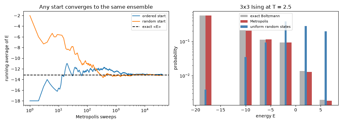
ordered start: <E> = -13.0581  (exact -13.1591)
random start: <E> = -13.1855  (exact -13.1591)

Check

Detailed balance makes Metropolis sample exp(-beta E) from any start.

assert np.sum(degeneracy) == 2**N
assert np.max(np.abs(hist["random start"] - p_exact)) < 0.01
assert abs(traces["random start"][-1] - E_exact) < 0.15 and abs(traces["ordered start"][-1] - E_exact) < 0.15