The Swendsen-Wang algorithm: flipping every Fortuin-Kasteleyn cluster at once

Swendsen and Wang (1987) used the Fortuin-Kasteleyn mapping of the Ising model onto bond percolation to build the first cluster Monte Carlo move. Every bond between two aligned neighbors is activated with probability

\[p = 1 - e^{-2\beta J},\]

the connected components of the activated bonds are the clusters, and each cluster is flipped independently with probability 1/2. One update resamples the whole lattice. This example shows the cluster decomposition of one configuration at \(T_C\), and compares how fast the energy decorrelates under Swendsen-Wang and under single-spin Metropolis at \(T_C\) on an \(L = 32\) lattice.

import matplotlib.pyplot as plt
import numpy as np
from scipy.ndimage import label

from physicskit.statphys.chapters.ising_lattice import Ising2D
from physicskit.statphys.core.monte_carlo import seed_numba_random
from physicskit.statphys.utils.dynamics import autocorrelation_function, integrated_autocorrelation_time

L = 32
model = Ising2D(L=L, seed=0)
beta = 1.0 / model.T_C
model.sweep(beta, algorithm="swendsen-wang", n_sweeps=200)

103

Fortuin-Kasteleyn clusters of one configuration

The bond activation is redrawn here in NumPy only to colour the clusters; the update itself runs in swendsen_wang_step_ising(). The activated bonds are drawn on a doubled grid, so neighbouring sites joined by a bond share one connected region.

rng = np.random.default_rng(1)
s = model.spins
p_bond = 1.0 - np.exp(-2.0 * beta * model.J)
grid = np.zeros((2 * L, 2 * L), dtype=bool)
grid[::2, ::2] = True
down = (s == np.roll(s, -1, axis=0)) & (rng.random((L, L)) < p_bond)
right = (s == np.roll(s, -1, axis=1)) & (rng.random((L, L)) < p_bond)
grid[1::2, ::2] = down
grid[::2, 1::2] = right
labels, n_clusters = label(grid, structure=[[0, 1, 0], [1, 1, 1], [0, 1, 0]])
site_labels = labels[::2, ::2]
print(f"{n_clusters} clusters (open boundaries in this picture), largest has {np.bincount(site_labels.ravel())[1:].max()} sites")

fig, axes = plt.subplots(1, 3, figsize=(13, 4.2))
axes[0].imshow(s, cmap="gray", interpolation="nearest")
axes[0].set_title(r"Spins at $T_C$")
shuffled = np.random.default_rng(2).permutation(n_clusters + 1)
axes[1].imshow(shuffled[site_labels], cmap="tab20", interpolation="nearest")
axes[1].set_title(f"Fortuin-Kasteleyn clusters, $p = 1 - e^{{-2\\beta J}} = {p_bond:.3f}$")
for ax in axes[:2]:
    ax.set_xticks([])
    ax.set_yticks([])

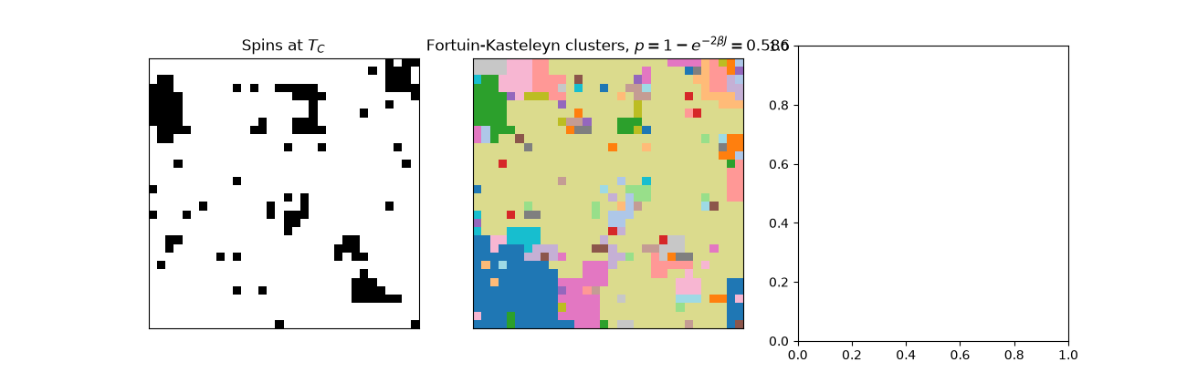
127 clusters (open boundaries in this picture), largest has 609 sites

Energy autocorrelation: Swendsen-Wang against Metropolis

n_samples = 4000
taus = {}
for algorithm, color in [("metropolis", "steelblue"), ("swendsen-wang", "darkorange")]:
    seed_numba_random(3)
    m = Ising2D(L=L, seed=3)
    m.sweep(beta, algorithm=algorithm, n_sweeps=500)
    E = np.empty(n_samples)
    for k in range(n_samples):
        m.sweep(beta, algorithm=algorithm, n_sweeps=1)
        E[k] = m.energy()
    taus[algorithm] = integrated_autocorrelation_time(E)
    rho = autocorrelation_function(E, max_lag=60)
    axes[2].plot(rho, color=color, label=rf"{algorithm}, $\tau_{{\rm int}} = {taus[algorithm]:.1f}$ sweeps")
    print(f"{algorithm}: tau_int(E) = {taus[algorithm]:.1f} sweeps")
axes[2].axhline(0.0, color="gray", lw=0.5)
axes[2].set_xlabel("lag (sweeps or cluster updates)")
axes[2].set_ylabel("energy autocorrelation")
axes[2].set_title(f"Decorrelation at $T_C$, L={L}")
axes[2].legend(fontsize=8)
plt.tight_layout()
plt.show()

metropolis: tau_int(E) = 132.6 sweeps
swendsen-wang: tau_int(E) = 9.4 sweeps

Check

Swendsen-Wang decorrelates the energy at \(T_C\) several times faster.

assert taus["swendsen-wang"] < taus["metropolis"] / 3