Alder and Wainwright: molecular dynamics simulation

In 1957 Alder and Wainwright took a different route from Monte Carlo: integrate Newton’s equations for a few hundred interacting particles and read equilibrium properties directly off the trajectory. Their simulations found that hard spheres with no attraction at all freeze into a crystal when packed densely enough. Order came from geometry alone.

This example runs the same kind of experiment with LennardJonesGas, which integrates lj_forces() with the time-reversible Velocity Verlet scheme (velocity_verlet_step()). It checks that the total energy is conserved, as a microcanonical simulation requires, and far better than with a naive Euler step. It then compares the pair distribution function \(g(r)\) of a dilute gas with that of a dense system, whose sharp shells reveal a solid.

import matplotlib.pyplot as plt
import numpy as np

from physicskit.statphys.chapters.molecular_dynamics import LennardJonesGas
from physicskit.statphys.core.md_engine import lj_forces

N = 144


def make_gas(density, T0, seed=1957):
    box = np.sqrt(N / density)
    return LennardJonesGas(n_particles=N, box_size=box, temperature_init=T0, dt=0.004, initial_velocity_distribution="maxwell_boltzmann", seed=seed)


def pair_distribution(positions, box, r_max, bins=120):
    d = positions[:, None, :] - positions[None, :, :]
    d -= box * np.round(d / box)
    r = np.sqrt((d**2).sum(-1))[np.triu_indices(len(positions), 1)]
    hist, edges = np.histogram(r, bins=bins, range=(0, r_max))
    shell = np.pi * (edges[1:] ** 2 - edges[:-1] ** 2)
    ideal = shell * len(positions) * (len(positions) - 1) / 2 / box**2
    return 0.5 * (edges[1:] + edges[:-1]), hist / ideal

Energy conservation: Verlet vs Euler

Same dense system, same time step. The time-reversible Verlet energy stays within about a percent (the small steps come from pairs crossing the interaction cutoff); forward Euler pumps energy in until particles are thrown into each other’s cores and the simulation explodes.

gas = make_gas(0.7, 0.6)
E_verlet = []
for _ in range(400):
    gas.step(5)
    E_verlet.append(gas.total_energy())
E_verlet = np.array(E_verlet)

euler = make_gas(0.7, 0.6)
x, v = euler.positions.copy(), euler.velocities.copy()
E_euler = []
for k in range(2000):
    F, U = lj_forces(x, euler.box_size)
    if k % 5 == 4:
        E_euler.append(0.5 * np.sum(v**2) + U)
    x = np.mod(x + v * euler.dt, euler.box_size)
    v = v + F * euler.dt
E_euler = np.array(E_euler)
print(f"Verlet: relative energy drift over 2000 steps {abs(E_verlet[-1] - E_verlet[0]) / abs(E_verlet[0]):.1e}")
print(f"Euler:  relative energy drift over 2000 steps {abs(E_euler[-1] - E_euler[0]) / abs(E_euler[0]):.1e}")

Verlet: relative energy drift over 2000 steps 8.0e-03
Euler:  relative energy drift over 2000 steps 4.8e+57

Structure from dynamics: gas vs solid

Equilibrate a dilute gas and a dense system, then average \(g(r)\) over the trajectory. The gas shows one weak neighbour peak and then nothing. The dense system shows sharp shells at the spacings of a triangular crystal, \(r_1\), \(\sqrt3 r_1\) and \(2r_1\). The dense system starts on a square lattice, which is not its lowest energy state; as it rearranges into a triangular one it releases energy and warms up, so its temperature is reported as measured.

results = {}
for label, density, T0 in [("dilute gas, rho = 0.05", 0.05, 1.0), ("dense, rho = 0.9", 0.9, 0.3)]:
    sim = make_gas(density, T0)
    sim.step(1500)
    g_acc, temps = 0, []
    for _ in range(40):
        sim.step(25)
        r, g = pair_distribution(sim.positions, sim.box_size, r_max=4.0)
        g_acc = g_acc + g / 40
        temps.append(sim.temperature())
    results[f"{label}, T = {np.mean(temps):.2f}"] = (r, g_acc, sim.positions.copy(), sim.box_size)
    print(f"{label}: kinetic temperature {np.mean(temps):.3f} +/- {np.std(temps):.3f}")
dense_key = [key for key in results if key.startswith("dense")][0]
r1 = results[dense_key][0][np.argmax(results[dense_key][1])]
print(f"dense system: first peak r1 = {r1:.3f}; triangular-lattice shells expected at {r1 * np.sqrt(3):.3f} and {2 * r1:.3f}")

fig, (ax1, ax2, ax3) = plt.subplots(1, 3, figsize=(15, 4))
ax1.semilogy(np.arange(len(E_verlet)) * 5 * gas.dt, np.abs(E_verlet / E_verlet[0] - 1) + 1e-16, color="steelblue", label="Velocity Verlet")
ax1.semilogy(np.arange(len(E_euler)) * 5 * euler.dt, np.abs(E_euler / E_euler[0] - 1) + 1e-16, color="firebrick", label="forward Euler")
ax1.set_xlabel("time")
ax1.set_ylabel(r"$|E(t)/E(0) - 1|$")
ax1.set_title("Microcanonical energy conservation")
ax1.legend(fontsize=8)
for label, (r, g, _, _) in results.items():
    ax2.plot(r, g, label=label)
for shell in (r1, np.sqrt(3) * r1, 2 * r1):
    ax2.axvline(shell, color="0.6", ls=":", lw=0.8)
ax2.set_xlabel("r / sigma")
ax2.set_ylabel("g(r)")
ax2.set_title("Pair distribution function")
ax2.legend(fontsize=8)
_, _, pos, box = results[dense_key]
ax3.plot(pos[:, 0], pos[:, 1], "o", ms=6, color="darkorchid")
ax3.set_xlim(0, box)
ax3.set_ylim(0, box)
ax3.set_aspect("equal")
ax3.set_title("Dense system: a crystal")
fig.tight_layout()

plt.show()

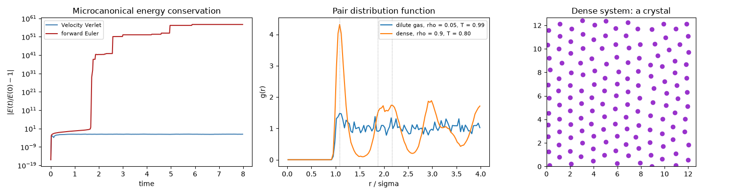
dilute gas, rho = 0.05: kinetic temperature 0.989 +/- 0.018
dense, rho = 0.9: kinetic temperature 0.795 +/- 0.041
dense system: first peak r1 = 1.083; triangular-lattice shells expected at 1.876 and 2.167

Check

Velocity Verlet conserves energy to < 2%; forward Euler explodes. The dilute gas keeps its temperature; the dense system crystallizes with its first neighbour at the triangular-lattice spacing sqrt(2 / (sqrt(3) rho)).

assert abs(E_verlet[-1] - E_verlet[0]) / abs(E_verlet[0]) < 0.02
assert abs(E_euler[-1] - E_euler[0]) / abs(E_euler[0]) > 1
assert abs(r1 - np.sqrt(2 / (np.sqrt(3) * 0.9))) < 0.07