
Note
Go to the end to download the full example code.
Boltzmann’s H-theorem: relaxation to the Maxwell-Boltzmann distribution#
This example simulates a 2D periodic gas of \(N=200\) particles interacting pairwise through the Lennard-Jones potential
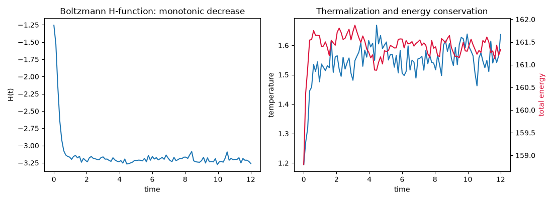
integrated forward with the symplectic Velocity Verlet scheme. Boltzmann’s H-theorem is one of the most celebrated (and originally controversial) results in statistical mechanics: even though this underlying Newtonian dynamics is perfectly time-reversible, the coarse-grained velocity distribution evolves irreversibly toward the Maxwell-Boltzmann equilibrium form, with the H-function
(Boltzmann’s \(\int f \ln f \, d^2v\) written in terms of the speed distribution \(f(v)\), with \(2\pi v\) the 2D Jacobian) decreasing monotonically on average as the gas thermalizes, since the Maxwell-Boltzmann distribution is the one that minimizes \(H\) at fixed energy. This example starts the gas from a highly artificial “delta-function” speed distribution – every particle moving at the same speed, in a random direction – and watches it relax.
import matplotlib.pyplot as plt
import numpy as np
from scipy.stats import kurtosis

from physicskit.statphys.chapters.molecular_dynamics import LennardJonesGas
from physicskit.statphys.visualizers.particle_render import plot_velocity_histogram
Relax a far-from-equilibrium gas and track H(t)#
gas = LennardJonesGas(
    n_particles=200,
    box_size=25.0,
    temperature_init=1.2,
    initial_velocity_distribution="delta",
    dt=0.003,
    seed=0,
)
history = gas.run(n_steps=4000, steps_per_record=40)

fig, axes = plt.subplots(1, 2, figsize=(11, 4))
axes[0].plot(history["time"], history["H"])
axes[0].set_xlabel("time")
axes[0].set_ylabel("H(t)")
axes[0].set_title("Boltzmann H-function: monotonic decrease")

axes[1].plot(history["time"], history["temperature"], label="temperature")
ax2 = axes[1].twinx()
ax2.plot(history["time"], history["total_energy"], color="crimson", label="total energy")
axes[1].set_xlabel("time")
axes[1].set_ylabel("temperature")
ax2.set_ylabel("total energy", color="crimson")
axes[1].set_title("Thermalization and energy conservation")
plt.tight_layout()
Initial vs. final speed distribution against Maxwell-Boltzmann#
fig, ax = plt.subplots(figsize=(6, 4))
plot_velocity_histogram(gas, ax=ax)
ax.set_title(f"Final speed distribution (t = {gas.time:.1f})")
plt.tight_layout()
plt.show()
Check#
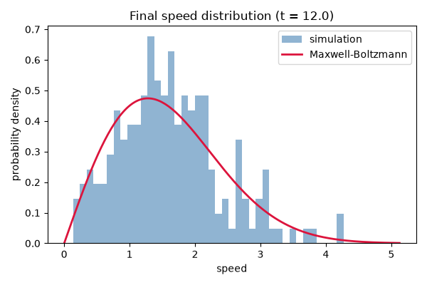
From equal speeds the gas relaxes to Maxwell-Boltzmann: H falls to the 2D equilibrium value -1 - ln(2 pi k_B T / m), each velocity component becomes Gaussian (zero excess kurtosis), and the total energy stays conserved.
Total running time of the script: (0 minutes 0.283 seconds)