Maxwell’s distribution of molecular velocities

Maxwell (1860) derived the distribution of molecular velocities in a gas without following a single molecule. He assumed only two things. The three velocity components are statistically independent, \(f(\mathbf v)=\phi(v_x)\phi(v_y)\phi(v_z)\), and no direction is special, so \(f\) depends only on \(|\mathbf v|\). The only function satisfying both is a Gaussian, which gives the speed distribution

\[f(v) = 4\pi v^2\left(\frac{m}{2\pi k_BT}\right)^{3/2}e^{-mv^2/2k_BT}.\]

This example shows why independence plus isotropy forces the Gaussian, then evaluates maxwell_boltzmann_speed_pdf() for nitrogen at several temperatures. It checks the characteristic speeds against sampled molecules, and compares the speed distributions in one, two and three dimensions.

import matplotlib.pyplot as plt
import numpy as np
from scipy.integrate import quad

from physicskit.constants import K_B
from physicskit.statphys.utils.thermodynamics import maxwell_boltzmann_component_pdf, maxwell_boltzmann_speed_pdf

Independence plus isotropy forces a Gaussian

Take the same one-component law for \(v_x\) and \(v_y\) and form the product. Only the Gaussian gives circular contours, i.e. a joint distribution that is the same in every direction. Uniform or exponential components give squares and diamonds.

v = np.linspace(-3, 3, 301)
VX, VY = np.meshgrid(v, v)
components = {
    "Gaussian": lambda u: np.exp(-(u**2) / 2),
    "uniform": lambda u: (np.abs(u) < 1.7).astype(float),
    "exponential": lambda u: np.exp(-np.abs(u) * 1.2),
}
fig1, axes = plt.subplots(1, 3, figsize=(12, 3.9))
for ax, (name, phi) in zip(axes, components.items()):
    joint = phi(VX) * phi(VY)
    ax.contour(VX, VY, joint, levels=6, cmap="viridis")
    ax.set_aspect("equal")
    ax.set_title(f"{name} components")
    ax.set_xlabel("$v_x$")
    ax.set_ylabel("$v_y$")
    th = np.linspace(0, 2 * np.pi, 720, endpoint=False)
    on_circle = phi(2.0 * np.cos(th)) * phi(2.0 * np.sin(th))
    spread = on_circle.std() / on_circle.mean()
    print(f"{name:12s}: relative variation of f around the circle |v| = 2: {spread:.3f}")
fig1.suptitle(r"$\phi(v_x)\,\phi(v_y)$: only the Gaussian is isotropic")
fig1.tight_layout()

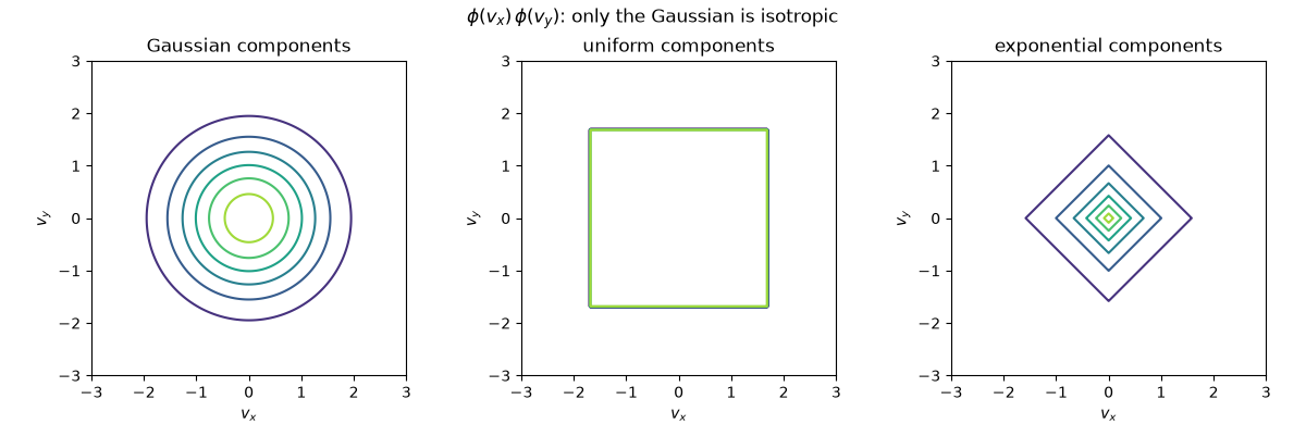
Gaussian    : relative variation of f around the circle |v| = 2: 0.000
uniform     : relative variation of f around the circle |v| = 2: 1.548
exponential : relative variation of f around the circle |v| = 2: 0.323

Nitrogen at three temperatures

Most probable, mean and rms speeds are in the fixed ratios \(\sqrt2 : \sqrt{8/\pi} : \sqrt3\), all scaling as \(\sqrt{T/m}\). Sampling 200,000 molecules as three independent Gaussian components reproduces them.

m_N2 = 28.0134 * 1.66053907e-27
rng = np.random.default_rng(1860)
speeds = np.linspace(0, 2500, 600)
fig2, (ax1, ax2) = plt.subplots(1, 2, figsize=(11, 4))
for T, color in [(100, "steelblue"), (300, "darkorange"), (1000, "firebrick")]:
    pdf = maxwell_boltzmann_speed_pdf(speeds, T, mass=m_N2, kB=K_B, dim=3)
    ax1.plot(speeds, pdf * 1e3, color=color, label=f"T = {T} K")
    sigma = np.sqrt(K_B * T / m_N2)
    sample = np.linalg.norm(rng.normal(0, sigma, (200_000, 3)), axis=1)
    print(
        f"T = {T:4d} K: v_p = {np.sqrt(2) * sigma:6.1f}, <v> = {np.sqrt(8 / np.pi) * sigma:6.1f} (sampled {sample.mean():6.1f}), "
        f"v_rms = {np.sqrt(3) * sigma:6.1f} (sampled {np.sqrt(np.mean(sample**2)):6.1f}) m/s"
    )
norm = quad(lambda s: maxwell_boltzmann_speed_pdf(s, 300, mass=m_N2, kB=K_B, dim=3), 0, 5000)[0]
print(f"normalization of f(v) at 300 K: {norm:.6f}")
ax1.set_xlabel("speed [m/s]")
ax1.set_ylabel(r"$f(v)$ [$10^{-3}$ s/m]")
ax1.set_title(r"Maxwell distribution for N$_2$")
ax1.legend(fontsize=8)

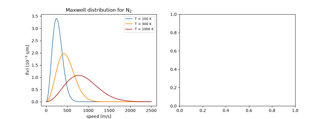
T =  100 K: v_p =  243.6, <v> =  274.9 (sampled  275.2), v_rms =  298.4 (sampled  298.6) m/s
T =  300 K: v_p =  422.0, <v> =  476.2 (sampled  476.3), v_rms =  516.8 (sampled  517.0) m/s
T = 1000 K: v_p =  770.5, <v> =  869.4 (sampled  869.2), v_rms =  943.6 (sampled  943.9) m/s
normalization of f(v) at 300 K: 1.000000

<matplotlib.legend.Legend object at 0x1700ce3f0>

One, two and three dimensions

The same Gaussian components give different speed distributions because the number of velocity directions with a given speed grows as \(v^{d-1}\). The one-component law itself, maxwell_boltzmann_component_pdf(), is the same in every case.

u = np.linspace(0, 4, 300)
for dim, ls in [(1, ":"), (2, "--"), (3, "-")]:
    ax2.plot(u, maxwell_boltzmann_speed_pdf(u, 1.0, dim=dim), "k", ls=ls, label=f"speed, d = {dim}")
ax2.plot(u, maxwell_boltzmann_component_pdf(u, 1.0), color="steelblue", alpha=0.5, lw=4, label=r"one component $\phi(v_x)$")
ax2.set_xlabel(r"$v / \sqrt{k_BT/m}$")
ax2.set_title("Speed distributions by dimension")
ax2.legend(fontsize=8)
fig2.tight_layout()

plt.show()

Check

Only Gaussian components give a rotation-invariant joint distribution (Maxwell’s argument); the speed distribution is normalized, and the sampled mean and rms speeds match sqrt(8/pi) sigma and sqrt(3) sigma.

phi_gauss = components["Gaussian"]
on_circle = phi_gauss(2.0 * np.cos(th)) * phi_gauss(2.0 * np.sin(th))
assert on_circle.std() / on_circle.mean() < 1e-12
assert abs(norm - 1) < 1e-6
assert abs(sample.mean() / (np.sqrt(8 / np.pi) * sigma) - 1) < 0.005
assert abs(np.sqrt(np.mean(sample**2)) / (np.sqrt(3) * sigma) - 1) < 0.005