Diffusion, the Einstein relation, and the central limit theorem

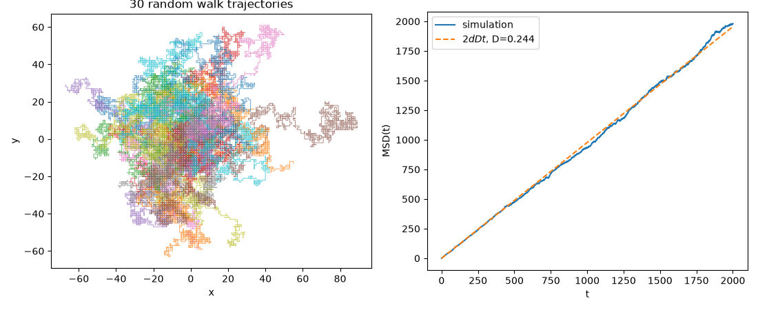
Einstein’s 1905 analysis of Brownian motion related a microscopically invisible quantity – the erratic jostling of a pollen grain by individual water molecules – to a macroscopically measurable one, the diffusion coefficient \(D\), via \(\langle r^2(t) \rangle = 2 d D t\) in \(d\) spatial dimensions. This was the first quantitative link between atomic-scale motion and observable matter, and it played a central role in convincing skeptics that atoms were real. This example simulates an ensemble of 500 independent walkers on a 2D lattice, each taking unit steps along a randomly chosen axis at every time step, recovers \(D\) from their mean squared displacement, and separately shows the central limit theorem in action: however non-Gaussian the individual steps are, the distribution of the walkers’ displacement after many steps is Gaussian.

import matplotlib.pyplot as plt
import numpy as np

from physicskit.statphys.chapters.random_walk import RandomWalk
from physicskit.statphys.visualizers.random_walk_render import (
    plot_clt_histogram,
    plot_msd,
    plot_trajectories_2d,
)

Trajectories and the Einstein relation

walk = RandomWalk(n_walkers=500, n_steps=2000, dim=2, kind="lattice", seed=0)
walk.run()

fig, axes = plt.subplots(1, 2, figsize=(11, 4.5))
plot_trajectories_2d(walk, ax=axes[0], n_show=30)
plot_msd(walk, ax=axes[1])
plt.tight_layout()

The central limit theorem

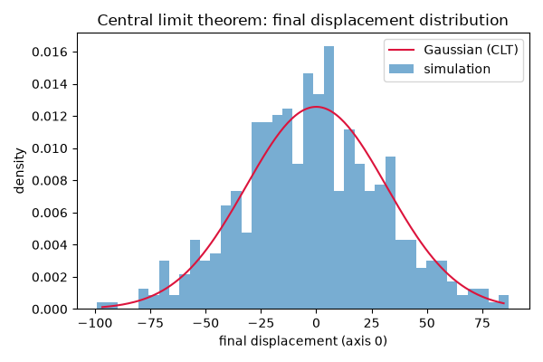
Even though each lattice-walk step is a discrete jump along a random axis – about as non-Gaussian a single-step distribution as one can construct – the distribution of the walker’s position after many steps is indistinguishable from a Gaussian.

fig, ax = plt.subplots(figsize=(6, 4))
plot_clt_histogram(walk, ax=ax, axis=0, bins=40)
ax.set_title("Central limit theorem: final displacement distribution")
plt.tight_layout()

The central limit theorem, caught in the act

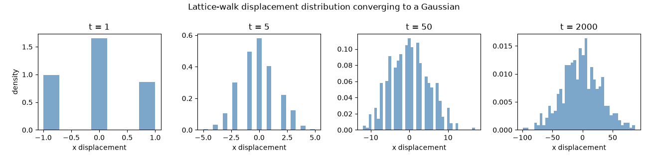
Rather than jumping straight to the final-time histogram above, the same already-simulated trajectories let the convergence itself be watched directly: after a single step the displacement distribution is just three discrete spikes (+1, -1, or 0 along this axis, from the two other lattice directions), and it visibly smooths into the continuous bell curve predicted by the CLT as more steps accumulate.

snapshot_steps = [1, 5, 50, walk.n_steps]
fig, axes = plt.subplots(1, len(snapshot_steps), figsize=(13, 3.2))
for ax, t in zip(axes, snapshot_steps):
    displacement_t = walk.trajectories[t, :, 0]
    bins = min(40, len(np.unique(displacement_t)) * 2 + 1)
    ax.hist(displacement_t, bins=bins, density=True, color="steelblue", alpha=0.7)
    ax.set_title(f"t = {t}")
    ax.set_xlabel("x displacement")
axes[0].set_ylabel("density")
plt.suptitle("Lattice-walk displacement distribution converging to a Gaussian")
plt.tight_layout()
plt.show()