The Langevin equation: Brownian motion one trajectory at a time

Langevin (1908) wrote Newton’s law for a single Brownian particle, splitting the fluid’s effect into a drag and a random kick:

\[m\frac{dv}{dt} = -\gamma v + \xi(t),\qquad \langle\xi(t)\xi(t')\rangle = 2\gamma k_BT\,\delta(t-t').\]

The noise strength is tied to the same friction that damps the motion. That balance guarantees equipartition, \(\langle v^2\rangle = k_BT/m\) in each direction, and it turns into Einstein’s diffusion constant \(D=k_BT/\gamma\). This example integrates the equation for 2000 independent particles with the Euler-Maruyama scheme. It checks equipartition, the exponential velocity memory \(\langle v(0)v(t)\rangle = (k_BT/m)e^{-\gamma t/m}\), and the crossover of the mean-squared displacement from ballistic \((k_BT/m)t^2\) at short times to diffusive \(2Dt\) at long times, which no diffusion-equation picture can show.

import matplotlib.pyplot as plt
import numpy as np

m, gamma, kT = 1.0, 2.0, 0.5
tau_v = m / gamma
D = kT / gamma
dt, n_steps, n_particles = 0.005, 4000, 2000
rng = np.random.default_rng(1908)

Integrate the Langevin equation

Start every particle at rest at the origin: velocities must first thermalize to the bath.

x = np.zeros(n_particles)
v = np.zeros(n_particles)
xs, vs = np.empty((n_steps + 1, n_particles)), np.empty((n_steps + 1, n_particles))
xs[0], vs[0] = x, v
kick = np.sqrt(2 * gamma * kT * dt) / m
for k in range(n_steps):
    v = v - gamma / m * v * dt + kick * rng.standard_normal(n_particles)
    x = x + v * dt
    xs[k + 1], vs[k + 1] = x, v
t = np.arange(n_steps + 1) * dt

Equipartition and velocity memory

After a few relaxation times \(m/\gamma\) the velocity variance sits at \(k_BT/m\). The velocity autocorrelation, measured in the stationary part of the run, decays exponentially with that same time constant.

late = t > 10 * tau_v
print(f"<v^2> (late) = {np.mean(vs[late] ** 2):.4f}   k_B T / m = {kT / m:.4f}")
start = np.searchsorted(t, 10 * tau_v)
lags = np.arange(0, 400, 5)
vacf = np.array([np.mean(vs[start : start + 2000] * vs[start + lag : start + lag + 2000]) for lag in lags])
fit_tau = -1 / np.polyfit(lags * dt, np.log(vacf / vacf[0]), 1)[0]
print(f"velocity memory time: fitted {fit_tau:.3f}, m / gamma = {tau_v:.3f}")

<v^2> (late) = 0.4992   k_B T / m = 0.5000
velocity memory time: fitted 0.475, m / gamma = 0.500

From ballistic to diffusive

Particles starting at rest have the exact mean-squared displacement \(\langle x^2\rangle = 2D\left[t - 2\tau(1-e^{-t/\tau}) + \tfrac{\tau}{2}(1-e^{-2t/\tau})\right]\) with \(\tau=m/\gamma\): quadratic in \(t\) at first, linear with slope \(2D\) later.

msd = np.mean(xs**2, axis=1)
msd_exact = 2 * D * (t - 2 * tau_v * (1 - np.exp(-t / tau_v)) + 0.5 * tau_v * (1 - np.exp(-2 * t / tau_v)))
D_fit = np.polyfit(t[t > 10], msd[t > 10], 1)[0] / 2
D_green_kubo = np.sum(vacf) * 5 * dt - 0.5 * vacf[0] * 5 * dt  # trapezoid rule over the velocity memory
print(f"diffusion constant: Green-Kubo integral of <v(0)v(t)> {D_green_kubo:.4f}; MSD slope {D_fit:.4f} (2000 walkers, a few % noise)")
print(f"Einstein relation D = k_B T / gamma = {D:.4f}")

fig, (ax1, ax2, ax3) = plt.subplots(1, 3, figsize=(15, 4))
for i in range(5):
    ax1.plot(t, xs[:, i], lw=0.8)
ax1.set_xlabel("time")
ax1.set_ylabel("x")
ax1.set_title("Five Langevin trajectories")
ax2.semilogy(lags * dt, vacf / vacf[0], "o", ms=3, color="steelblue", label="simulated")
ax2.semilogy(lags * dt, np.exp(-lags * dt / tau_v), "--", color="orange", label=r"$e^{-\gamma t/m}$")
ax2.set_xlabel("lag t")
ax2.set_ylabel(r"$\langle v(0)v(t)\rangle / \langle v^2\rangle$")
ax2.set_title("Velocity memory")
ax2.legend(fontsize=8)
ax3.loglog(t[1:], msd[1:], color="steelblue", label="simulated")
ax3.loglog(t[1:], msd_exact[1:], "k--", lw=1, label="exact")
ax3.loglog(t[1:50], (kT / m) * t[1:50] ** 2, ":", color="firebrick", label=r"ballistic $(k_BT/m)t^2$")
ax3.loglog(t[200:], 2 * D * t[200:], ":", color="darkgreen", label=r"diffusive $2Dt$")
ax3.set_xlabel("time")
ax3.set_ylabel(r"$\langle x^2\rangle$")
ax3.set_title("Mean-squared displacement")
ax3.legend(fontsize=8)
fig.tight_layout()

plt.show()

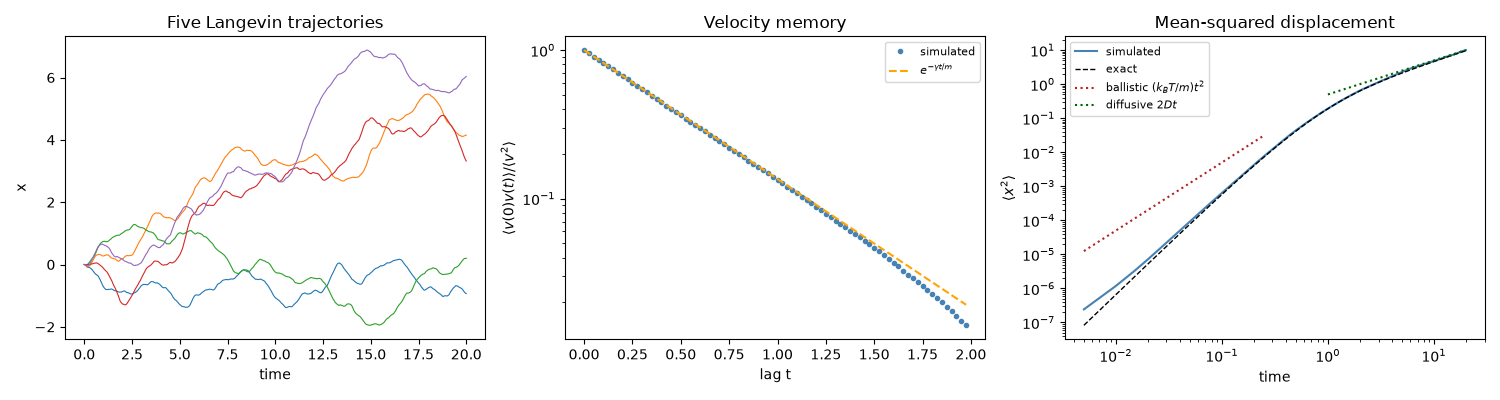
diffusion constant: Green-Kubo integral of <v(0)v(t)> 0.2436; MSD slope 0.2666 (2000 walkers, a few % noise)
Einstein relation D = k_B T / gamma = 0.2500

Check

Equipartition <v^2> = kT/m, velocity memory e^(-gamma t / m), and the Einstein relation D = kT / gamma from both Green-Kubo and the MSD.

assert abs(np.mean(vs[late] ** 2) / (kT / m) - 1) < 0.02
assert abs(fit_tau / tau_v - 1) < 0.1
assert abs(D_green_kubo / D - 1) < 0.1 and abs(D_fit / D - 1) < 0.1
assert np.max(np.abs(msd[t > 1] / msd_exact[t > 1] - 1)) < 0.1