The Ornstein-Uhlenbeck process: Gaussian noise with a memory

In 1930 George Uhlenbeck and Leonard Ornstein solved Langevin’s equation for the velocity of a free Brownian particle exactly. The velocity is not white noise. It is a process pulled back toward its mean at a rate \(\theta\) while being kicked with strength \(\sigma\),

\[dX = \theta(\mu - X)\,dt + \sigma\,dW.\]

From a fixed start its mean relaxes as \(e^{-\theta t}\) and its variance fills in as \(\frac{\sigma^2}{2\theta}(1 - e^{-2\theta t})\). Once stationary, it forgets its past exponentially, \(\langle \delta X(0)\,\delta X(\tau)\rangle = \frac{\sigma^2}{2\theta}e^{-\theta|\tau|}\). Doob (1942) later showed it is the only process that is at once stationary, Gaussian, and Markov.

OrnsteinUhlenbeck samples it with the exact Gaussian transition, or by Euler-Maruyama integration of the SDE. This example checks every one of these formulas, and shows the small, predictable bias that time stepping adds to the stationary variance.

import matplotlib.pyplot as plt
import numpy as np

from physicskit.statphys import OrnsteinUhlenbeck

theta, mu, sigma = 1.0, 0.0, 1.0

Relaxation from a fixed start

ou = OrnsteinUhlenbeck(theta=theta, mu=mu, sigma=sigma, n_paths=20000, seed=1930)
t, X = ou.run(t_max=5.0, dt=0.01, n_frames=250, x0=3.0)
print(f"stationary variance sigma^2 / 2 theta = {ou.stationary_variance:.4f}; sampled at t = 5: {X[-1].var():.4f}")

stationary variance sigma^2 / 2 theta = 0.5000; sampled at t = 5: 0.4924

Stationary memory

Starting from the stationary distribution, the autocovariance at lag \(\tau\) decays as \(e^{-\theta\tau}\): the process remembers its value for a time \(1/\theta\).

t_s, X_s = ou.run(t_max=5.0, dt=0.01, n_frames=100)
lags = np.arange(0, 60)
acov = np.array([np.mean((X_s[0] - mu) * (X_s[lag] - mu)) for lag in lags])

Time-step bias of Euler-Maruyama

The exact update has no time-step error. Euler-Maruyama overshoots the stationary variance by the factor \(1/(1 - \theta\Delta t/2)\), which is negligible for \(\theta\Delta t \ll 1\).

dts = np.array([0.02, 0.1, 0.25, 0.5, 1.0])
em_var = []
for dt in dts:
    em = OrnsteinUhlenbeck(theta=theta, mu=mu, sigma=sigma, n_paths=40000, seed=int(1000 * dt))
    _, Xe = em.run(t_max=8.0, dt=dt, n_frames=4, x0=0.0, method="euler_maruyama")
    em_var.append(Xe[-1].var())
    print(f"dt = {dt:4.2f}: Euler-Maruyama variance {em_var[-1]:.4f}, predicted {sigma**2 / (theta * (2 - theta * dt)):.4f}")

fig, axes = plt.subplots(1, 3, figsize=(15, 4.3))
for i in range(6):
    axes[0].plot(t, X[:, i], lw=0.6)
axes[0].plot(t, X.mean(axis=1), "k", lw=2, label="ensemble mean")
axes[0].plot(t, ou.mean(t, 3.0), "w--", lw=1)
sd = np.sqrt(ou.variance(t))
axes[0].fill_between(t, ou.mean(t, 3.0) - sd, ou.mean(t, 3.0) + sd, color="gray", alpha=0.3, label=r"exact mean $\pm$ sd")
axes[0].set_xlabel("t")
axes[0].set_ylabel("X")
axes[0].set_title("relaxing from X = 3")
axes[0].legend(fontsize=8)

axes[1].plot(t_s[lags], acov, "o", ms=3, label="sampled")
axes[1].plot(t_s[lags], ou.autocovariance(t_s[lags]), "k--", label=r"$\frac{\sigma^2}{2\theta}e^{-\theta\tau}$")
axes[1].set_xlabel(r"lag $\tau$")
axes[1].set_title("stationary autocovariance")
axes[1].legend()

axes[2].plot(dts, em_var, "o", label="Euler-Maruyama")
fine = np.linspace(0, 1.05, 100)
axes[2].plot(fine, sigma**2 / (theta * (2 - theta * fine)), "k--", lw=1, label=r"$\sigma^2/\theta(2-\theta\Delta t)$")
axes[2].axhline(ou.stationary_variance, color="gray", ls=":", label="exact")
axes[2].set_xlabel(r"$\theta\,\Delta t$")
axes[2].set_ylabel("stationary variance")
axes[2].set_title("time-step bias")
axes[2].legend()
fig.tight_layout()
plt.show()

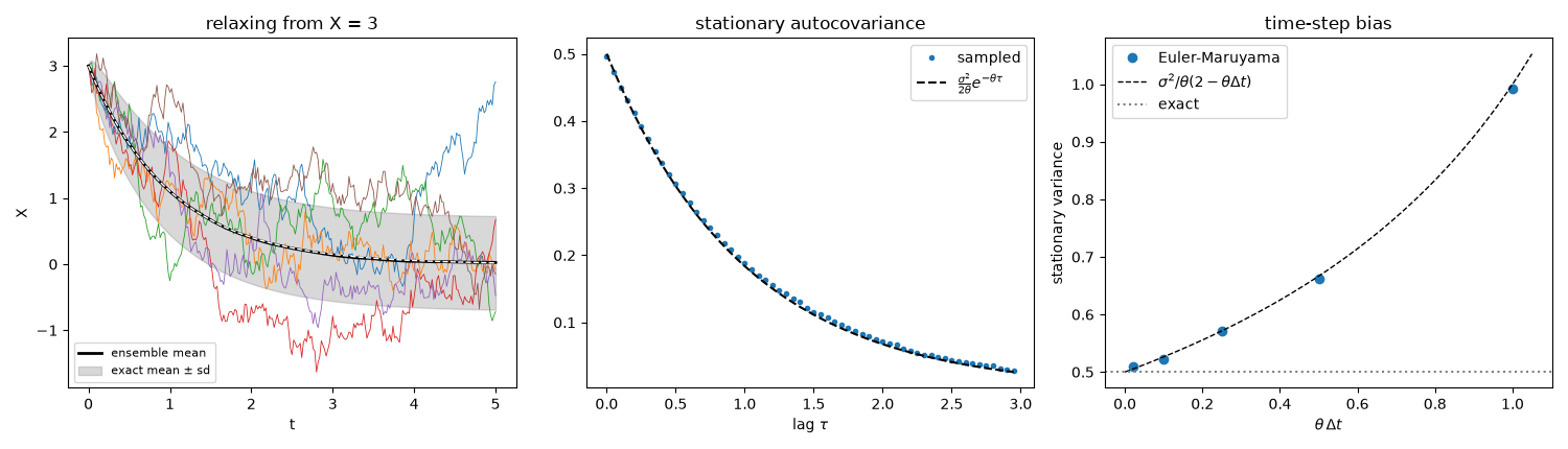
dt = 0.02: Euler-Maruyama variance 0.5093, predicted 0.5051
dt = 0.10: Euler-Maruyama variance 0.5225, predicted 0.5263
dt = 0.25: Euler-Maruyama variance 0.5714, predicted 0.5714
dt = 0.50: Euler-Maruyama variance 0.6619, predicted 0.6667
dt = 1.00: Euler-Maruyama variance 0.9916, predicted 1.0000

Check

Stationary variance sigma^2 / 2 theta, autocovariance e^(-theta tau), and the Euler-Maruyama bias sigma^2 / theta (2 - theta dt).

assert abs(X[-1].var() / ou.stationary_variance - 1) < 0.03
assert np.max(np.abs(acov - ou.autocovariance(t_s[lags]))) < 0.02
np.testing.assert_allclose(em_var, sigma**2 / (theta * (2 - theta * dts)), rtol=0.03)