Gibbs’s equilibrium criterion: minimum total Gibbs energy

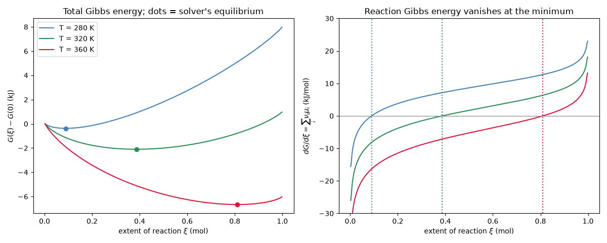
Gibbs showed that at fixed temperature and pressure a system reaches equilibrium at the minimum of its total Gibbs energy \(G = \sum_i n_i\mu_i\). For \(N_2O_4 \rightleftharpoons 2NO_2\) this example plots \(G(\xi)\) from gibbs_energy_of_mixture() at several temperatures and marks the composition returned by solve_equilibrium_composition(), which sits at each minimum. The slope \(dG/d\xi = \sum_i\nu_i\mu_i\) (the reaction Gibbs energy) crosses zero there.

import matplotlib.pyplot as plt
import numpy as np

from chemistrykit.thermo.systems.equilibrium import gibbs_energy_of_mixture, solve_equilibrium_composition

dH, dS = 57_200.0, 175.8  # N2O4 -> 2 NO2, J/mol and J/(mol K)
xi = np.linspace(0.002, 0.998, 400)

fig, axes = plt.subplots(1, 2, figsize=(12, 4.8))
for T, color in [(280.0, "steelblue"), (320.0, "seagreen"), (360.0, "crimson")]:
    gf = [0.0, (dH - T * dS) / 2.0]
    G = np.array([gibbs_energy_of_mixture([1 - x, 2 * x], gf, T) for x in xi])
    res = solve_equilibrium_composition(("N2O4", "NO2"), [[-1.0], [2.0]], [1.0, 0.0], gf, T)
    G_eq = gibbs_energy_of_mixture(res.n, gf, T)
    axes[0].plot(xi, (G - G[0]) / 1000.0, color=color, label=f"T = {T:.0f} K")
    axes[0].plot(res.extents[0], (G_eq - G[0]) / 1000.0, "o", color=color)
    axes[1].plot(xi, np.gradient(G, xi) / 1000.0, color=color)
    axes[1].axvline(res.extents[0], color=color, linestyle=":")
axes[0].set_xlabel(r"extent of reaction $\xi$ (mol)")
axes[0].set_ylabel(r"$G(\xi) - G(0)$ (kJ)")
axes[0].set_title("Total Gibbs energy; dots = solver's equilibrium")
axes[0].legend()
axes[1].axhline(0.0, color="gray", linewidth=0.8)
axes[1].set_ylim(-30, 30)
axes[1].set_xlabel(r"extent of reaction $\xi$ (mol)")
axes[1].set_ylabel(r"$dG/d\xi = \sum_i \nu_i \mu_i$ (kJ/mol)")
axes[1].set_title("Reaction Gibbs energy vanishes at the minimum")
fig.tight_layout()

plt.show()