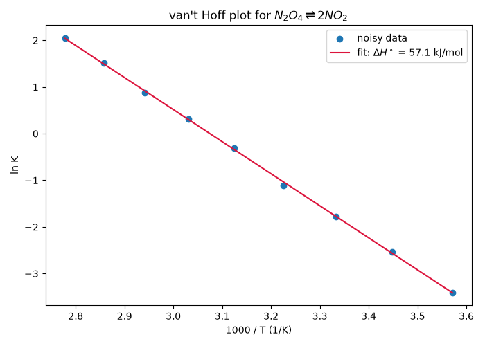
The van’t Hoff plot: ln K against 1/T

van’t Hoff’s equation \(d\ln K/dT = \Delta H^\circ/(RT^2)\) makes \(\ln K\) a straight line in \(1/T\) with slope \(-\Delta H^\circ/R\) and intercept \(\Delta S^\circ/R\). This example generates noisy equilibrium constants for \(N_2O_4 \rightleftharpoons 2NO_2\) from van_t_hoff_equilibrium_constant() and recovers the reaction enthalpy and entropy with fit_van_t_hoff().

import matplotlib.pyplot as plt
import numpy as np

from chemistrykit.constants import R
from chemistrykit.thermo.systems.equilibrium import fit_van_t_hoff, van_t_hoff_equilibrium_constant

dH_true, dS_true = 57_200.0, 175.8
T_ref = 298.15
K_ref = np.exp(-(dH_true - T_ref * dS_true) / (R * T_ref))

rng = np.random.default_rng(1)
T_data = np.linspace(280.0, 360.0, 9)
K_data = van_t_hoff_equilibrium_constant(T_data, T_ref=T_ref, K_ref=K_ref, delta_h=dH_true)
K_data = K_data * np.exp(rng.normal(scale=0.05, size=T_data.size))  # 5% multiplicative noise

fit = fit_van_t_hoff(T_data, K_data)

fig, ax = plt.subplots(figsize=(7, 5))
ax.scatter(1000.0 / T_data, np.log(K_data), label="noisy data")
T_line = np.linspace(T_data.min(), T_data.max(), 100)
ax.plot(1000.0 / T_line, np.log(fit.predict(T_line)), color="crimson", label=rf"fit: $\Delta H^\circ$ = {fit.delta_h / 1000:.1f} kJ/mol")
ax.set_xlabel("1000 / T (1/K)")
ax.set_ylabel("ln K")
ax.set_title(r"van't Hoff plot for $N_2O_4 \rightleftharpoons 2NO_2$")
ax.legend()
fig.tight_layout()

print(f"fitted dH = {fit.delta_h / 1000:.2f} kJ/mol (true {dH_true / 1000:.2f})")
print(f"fitted dS = {fit.delta_s:.1f} J/(mol K) (true {dS_true:.1f}); R^2 = {fit.r_squared:.4f}")

plt.show()

fitted dH = 57.14 kJ/mol (true 57.20)
fitted dS = 175.7 J/(mol K) (true 175.8); R^2 = 0.9996