Eddington’s mass-luminosity relation

Eddington (1924) showed that a main-sequence star’s luminosity is fixed almost entirely by its mass, regardless of what actually generates the star’s energy – fifteen years before Bethe worked out the nuclear reactions responsible:

\[\frac{L}{L_\odot} \approx \left(\frac{M}{M_\odot}\right)^{3.5}.\]

main_sequence_luminosity() implements exactly this power law. This example plots it across the 0.5-10 solar-mass range for which it is calibrated, contrasts its steep scaling against a naive linear guess (\(L\propto M\)), and shows why the relation makes a star’s lifetime fall steeply with mass: more massive stars burn dramatically brighter, but do not carry proportionally more fuel, so they exhaust it far faster.

import matplotlib.pyplot as plt
import numpy as np

from physicskit.astro.stellar_structure import main_sequence_luminosity

The mass-luminosity relation

mass_values = np.linspace(0.5, 10.0, 200)
luminosity = np.array([main_sequence_luminosity(m) for m in mass_values])
luminosity_linear = mass_values  # naive L ~ M guess, for contrast

print(f"L(1 solar mass)  = {main_sequence_luminosity(1.0):.4f} solar luminosities (the Sun, by construction)")
print(f"L(2 solar masses) = {main_sequence_luminosity(2.0):.4f} solar luminosities (a linear guess would give 2.0)")
print(f"L(10 solar masses) = {main_sequence_luminosity(10.0):.1f} solar luminosities (a linear guess would give 10.0)")

fig1, (ax1, ax2) = plt.subplots(1, 2, figsize=(11, 4.5))
ax1.loglog(mass_values, luminosity, color="steelblue", label=r"$L\propto M^{3.5}$ (Eddington)")
ax1.loglog(mass_values, luminosity_linear, "--", color="0.6", label=r"naive $L\propto M$")
ax1.set_xlabel(r"mass ($M_\odot$)")
ax1.set_ylabel(r"luminosity ($L_\odot$)")
ax1.set_title("Mass-luminosity relation (log-log)")
ax1.legend(fontsize=8)

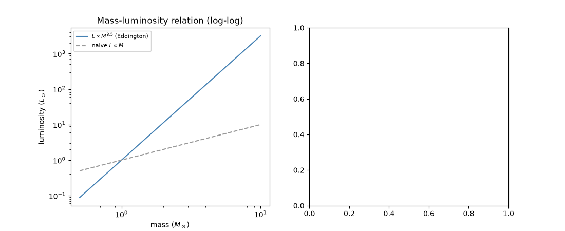
L(1 solar mass)  = 1.0000 solar luminosities (the Sun, by construction)
L(2 solar masses) = 11.3137 solar luminosities (a linear guess would give 2.0)
L(10 solar masses) = 3162.3 solar luminosities (a linear guess would give 10.0)

<matplotlib.legend.Legend object at 0x12482f350>

Consequence: stellar lifetime falls steeply with mass

A star’s nuclear fuel supply scales with its mass (roughly linearly), but it burns that fuel at a rate set by its luminosity, so its main-sequence lifetime scales as \(\tau\propto M/L\propto M^{1-3.5}=M^{-2.5}\) – a massive star burns dramatically brighter without carrying proportionally more fuel, so it lives dramatically shorter.

lifetime_relative = mass_values / luminosity  # relative to the Sun's own lifetime
ax2.loglog(mass_values, lifetime_relative, color="firebrick")
ax2.set_xlabel(r"mass ($M_\odot$)")
ax2.set_ylabel(r"lifetime, relative to the Sun's")
ax2.set_title(r"$\tau \propto M/L \propto M^{-2.5}$: massive stars live fast")
fig1.tight_layout()

relative_lifetime_10 = 10.0 / main_sequence_luminosity(10.0)
print(f"\nrelative lifetime at 10 solar masses: {relative_lifetime_10:.4f} (lives roughly {1 / relative_lifetime_10:.0f}x shorter than the Sun)")

plt.show()

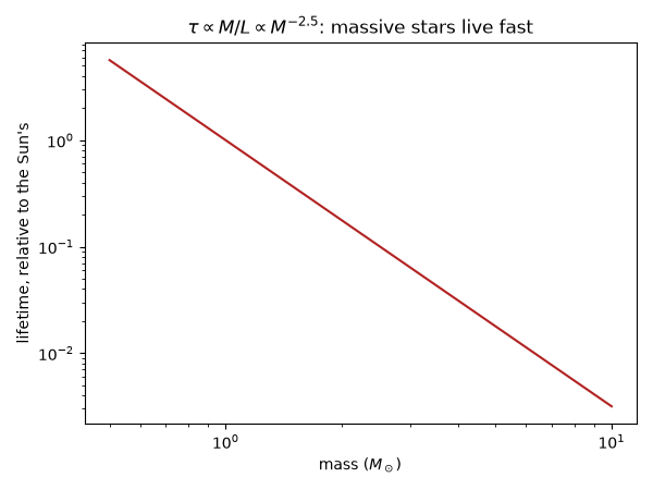
relative lifetime at 10 solar masses: 0.0032 (lives roughly 316x shorter than the Sun)