Liouville’s theorem: a swarm of pendulums

PendulumSwarm evolves \(N\) mutually independent, identical simple pendulums together as one separable Hamiltonian system, one pair \((q_i, p_i)\) per pendulum,

\[H = \sum_{i=1}^{N} \left[\frac{p_i^2}{2} - \frac{g}{l}\cos q_i\right] ,\]

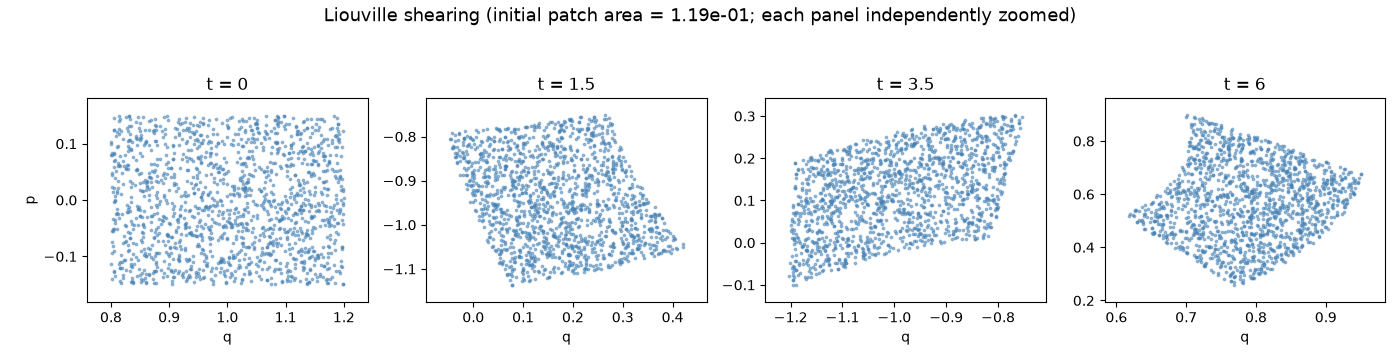
each obeying its own Hamilton’s equations independently. Liouville’s theorem states that the phase-space area (in general, volume) occupied by an ensemble of initial conditions is exactly conserved by Hamiltonian flow, even as the occupied region deforms arbitrarily. Here 1500 pendulums are seeded uniformly inside a small \((q, p)\) box and evolved together; the patch shears into a thin, filamented sliver while its area stays fixed. Each snapshot is independently zoomed to its own patch, since the whole patch also drifts through phase space as it deforms, and a shared/global view would make the (tiny, by comparison) internal shearing invisible – then the (convex-hull-estimated) patch area is tracked over a shorter window, before the shape becomes thin enough for that estimate to overstate the true conserved measure.

import matplotlib.pyplot as plt
import numpy as np
from matplotlib.animation import FuncAnimation

from physicskit.classical.systems.hamiltonian import PendulumSwarm


def _zoom_to_patch(ax, q, p, pad_frac=0.1):
    pad_q = pad_frac * (q.max() - q.min()) + 1e-3
    pad_p = pad_frac * (p.max() - p.min()) + 1e-3
    ax.set_xlim(q.min() - pad_q, q.max() + pad_q)
    ax.set_ylim(p.min() - pad_p, p.max() + pad_p)


def build_shearing_animation(n=1500, n_frames=120, t_final=6.0, dt=1e-3, seed=0):
    """A comoving-zoom animation of the swarm shearing continuously,
    rather than four disconnected snapshots -- returns a FuncAnimation."""
    swarm = PendulumSwarm.from_box(q_center=1.0, p_center=0.0, dq=0.4, dp=0.3, n=n, seed=seed)
    frame_times = np.linspace(0, t_final, n_frames)
    frames_q, frames_p = [swarm.q.copy()], [swarm.p.copy()]
    for t_target in frame_times[1:]:
        swarm.integrate((swarm.t, t_target), dt=dt, method="yoshida4")
        frames_q.append(swarm.q.copy())
        frames_p.append(swarm.p.copy())

    fig, ax = plt.subplots(figsize=(5.5, 5.3))
    scatter = ax.scatter(frames_q[0], frames_p[0], s=4, color="steelblue", alpha=0.6)
    ax.set_xlabel("q")
    ax.set_ylabel("p")
    title = ax.set_title(f"t = {frame_times[0]:.2f}\n(comoving zoom: the patch's own area never changes)")
    _zoom_to_patch(ax, frames_q[0], frames_p[0])
    fig.tight_layout()

    def update(i):
        scatter.set_offsets(np.column_stack([frames_q[i], frames_p[i]]))
        _zoom_to_patch(ax, frames_q[i], frames_p[i])
        title.set_text(f"t = {frame_times[i]:.2f}\n(comoving zoom: the patch's own area never changes)")
        return scatter, title

    return FuncAnimation(fig, update, frames=n_frames, interval=60, blit=False)

Watching the patch shear, continuously

anim = build_shearing_animation()

Four snapshots, each independently zoomed

swarm = PendulumSwarm.from_box(q_center=1.0, p_center=0.0, dq=0.4, dp=0.3, n=1500, seed=0)
area0 = swarm.phase_space_area()

snapshots = [(swarm.q.copy(), swarm.p.copy(), 0.0)]
for t_target in (1.5, 3.5, 6.0):
    swarm.integrate((swarm.t, t_target), dt=1e-3, method="yoshida4")
    snapshots.append((swarm.q.copy(), swarm.p.copy(), t_target))

fig1, axes = plt.subplots(1, 4, figsize=(14, 3.6))
for ax, (q, p, t) in zip(axes, snapshots):
    ax.scatter(q, p, s=3, color="steelblue", alpha=0.5)
    ax.set_title(f"t = {t:g}")
    ax.set_xlabel("q")
    _zoom_to_patch(ax, q, p)
axes[0].set_ylabel("p")
fig1.suptitle(f"Liouville shearing (initial patch area = {area0:.2e}; each panel independently zoomed)", fontsize=13)
fig1.tight_layout(rect=[0, 0, 1, 0.92])

Patch area tracked over a shorter, still-convex window

A smaller box than the visually dramatic one above: the convex-hull area estimate is more accurate for a nearly-convex patch, giving a tighter quantitative check of Liouville’s theorem.

swarm2 = PendulumSwarm.from_box(1.0, 0.0, 0.05, 0.05, n=500, seed=1)
areas, times = [swarm2.phase_space_area()], [0.0]
for _ in range(20):
    swarm2.integrate((swarm2.t, swarm2.t + 0.25), dt=1e-3, method="yoshida4")
    areas.append(swarm2.phase_space_area())
    times.append(swarm2.t)
print(f"area at t=0: {areas[0]:.4e}, area at t={times[-1]:.2f}: {areas[-1]:.4e} (ratio {areas[-1] / areas[0]:.4f})")

fig2, ax2 = plt.subplots(figsize=(6, 4))
ax2.plot(times, areas, "o-", color="firebrick")
ax2.axhline(areas[0], color="0.7", lw=0.8, ls="--")
ax2.set_xlabel("t")
ax2.set_ylabel("phase-space patch area")
ax2.set_title("Liouville's theorem: area is (nearly) constant")
fig2.tight_layout()

plt.show()

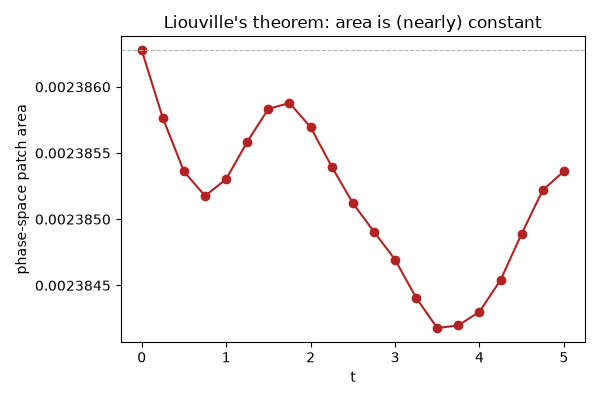
area at t=0: 2.3863e-03, area at t=5.00: 2.3854e-03 (ratio 0.9996)