Action-angle variables for the pendulum

For a 1-DOF system like the simple pendulum, \(H = p^2/2 - (g/l)\cos q\), every librating (bounded, non-circulating) orbit lies on a closed invariant curve in phase space labeled by a single number: the action

\[J(E) = \frac{1}{2\pi} \oint p \, dq ,\]

the phase-space area enclosed by that curve, divided by \(2\pi\). pendulum_action_angle() evaluates \(J(E)\) and the orbital period \(T(E)\) in closed form via complete elliptic integrals of the first and second kind, \(K(k)\) and \(E_{\mathrm{ellip}}(k)\): with \(k^2 = (E + g/l)/(2g/l)\),

\[J(E) = \frac{8}{\pi}\sqrt{\frac{g}{l}} \left[E_{\mathrm{ellip}}(k) - (1 - k^2) K(k)\right] , \qquad T(E) = \frac{4 K(k)}{\sqrt{g/l}} .\]

This plots both \(J(E)\) and \(T(E)\) as functions of energy, checks the small-oscillation limit (\(T \to 2\pi/\sqrt{g/l}\), the simple-harmonic-oscillator period, as \(E\) approaches the bottom of the well), and validates the predicted period directly against the measured period of an actually-integrated trajectory.

import matplotlib.pyplot as plt
import numpy as np

from physicskit.classical.systems.hamiltonian import PendulumSwarm, pendulum_action_angle

g_over_l = 1.0

J(E) and T(E) across the librating energy range

energies = np.linspace(-0.98, 0.98, 200) * g_over_l
actions = np.empty_like(energies)
periods = np.empty_like(energies)
for i, E in enumerate(energies):
    actions[i], periods[i] = pendulum_action_angle(E, g_over_l)

sho_period = 2 * np.pi / np.sqrt(g_over_l)
print(f"small-oscillation limit: measured T(E->-g/l) = {periods[0]:.4f}, SHO period 2*pi/sqrt(g/l) = {sho_period:.4f}")

fig1, axes = plt.subplots(1, 2, figsize=(10, 4.3))
axes[0].plot(energies, actions, color="steelblue")
axes[0].set_xlabel("E")
axes[0].set_ylabel("J(E)")
axes[0].set_title("Action grows monotonically with energy")

axes[1].plot(energies, periods, color="firebrick")
axes[1].axhline(sho_period, color="0.6", ls="--", lw=0.8, label="small-oscillation limit $2\\pi/\\sqrt{g/l}$")
axes[1].set_xlabel("E")
axes[1].set_ylabel("T(E)")
axes[1].set_title("Period diverges approaching the separatrix (E -> g/l)")
axes[1].legend(fontsize=9)
fig1.tight_layout()

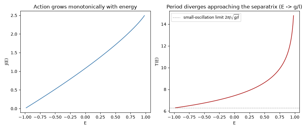
small-oscillation limit: measured T(E->-g/l) = 6.2990, SHO period 2*pi/sqrt(g/l) = 6.2832

Validate T(E) against an actually-integrated trajectory

fig2, ax2 = plt.subplots(figsize=(6.5, 5))
for E, color in [(-0.9, "steelblue"), (0.0, "darkorange"), (0.8, "firebrick")]:
    J, T_predicted = pendulum_action_angle(E, g_over_l)
    p0 = np.sqrt(2 * (E + g_over_l))
    system = PendulumSwarm(np.array([0.0]), np.array([p0]), g_over_l=g_over_l)
    result = system.integrate((0, 2 * T_predicted), dt=T_predicted / 2000, method="yoshida4")
    q = result.q[:, 0]
    crossing_idx = next(i for i in range(1, len(q)) if q[i - 1] < 0 <= q[i])
    T_measured = result.t[crossing_idx]
    print(f"E={E:+.1f}: predicted T={T_predicted:.4f}, measured T={T_measured:.4f}, J={J:.4f}")
    ax2.plot(result.q[:, 0], result.p[:, 0], color=color, label=f"E={E:+.1f}, J={J:.3f}")

theta = np.linspace(-np.pi, np.pi, 400)
ax2.plot(theta, np.sqrt(np.maximum(2 * (g_over_l + g_over_l * np.cos(theta)), 0)), color="0.6", ls="--", lw=1, label="separatrix (E=g/l)")
ax2.plot(theta, -np.sqrt(np.maximum(2 * (g_over_l + g_over_l * np.cos(theta)), 0)), color="0.6", ls="--", lw=1)
ax2.set_xlabel("q")
ax2.set_ylabel("p")
ax2.set_title("Each closed curve is one invariant torus, labeled by J")
ax2.legend(fontsize=9)
fig2.tight_layout()

plt.show()

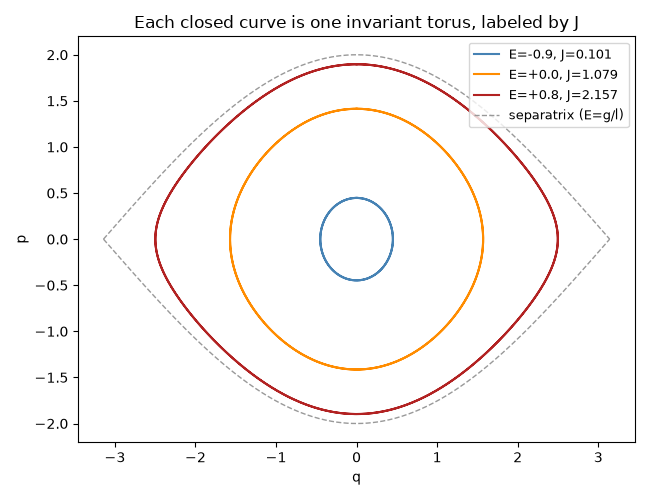
E=-0.9: predicted T=6.3640, measured T=6.3672, J=0.1006
E=+0.0: predicted T=7.4163, measured T=7.4200, J=1.0787
E=+0.8: predicted T=10.3124, measured T=10.3124, J=2.1568