Hamilton’s canonical (q, p) phase space

Lagrange’s mechanics lives in a “position and velocity” space (q, qdot); Hamilton’s 1834 reformulation trades each qdot for its canonically conjugate momentum p = dL/dqdot via a Legendre transform, and rewrites the second-order Euler-Lagrange equation as twice as many first-order equations for (q, p) moving through a single unified phase space:

\[\dot q = \frac{\partial H}{\partial p}, \qquad \dot p = -\frac{\partial H}{\partial q}\]

Two pendulums with very different-looking motion – one librating back and forth, one spinning all the way over the top – are, in this description, just two trajectories through the same canonical space, governed by the same H and separated by a single curve of constant energy: the separatrix. This shared (q, p) structure is exactly what HamiltonianSystem exposes, and what Liouville’s theorem (Liouville’s theorem: a swarm of pendulums) and symplectic integration (Why symplectic integration: RK4 leaks energy, Yoshida4 does not) both depend on.

import matplotlib.pyplot as plt
import numpy as np

from physicskit.classical.systems.hamiltonian import PendulumSwarm
from physicskit.classical.visualizers.phase_space import plot_phase_portrait

g_over_l = 1.0

One canonical system, two qualitatively different orbits

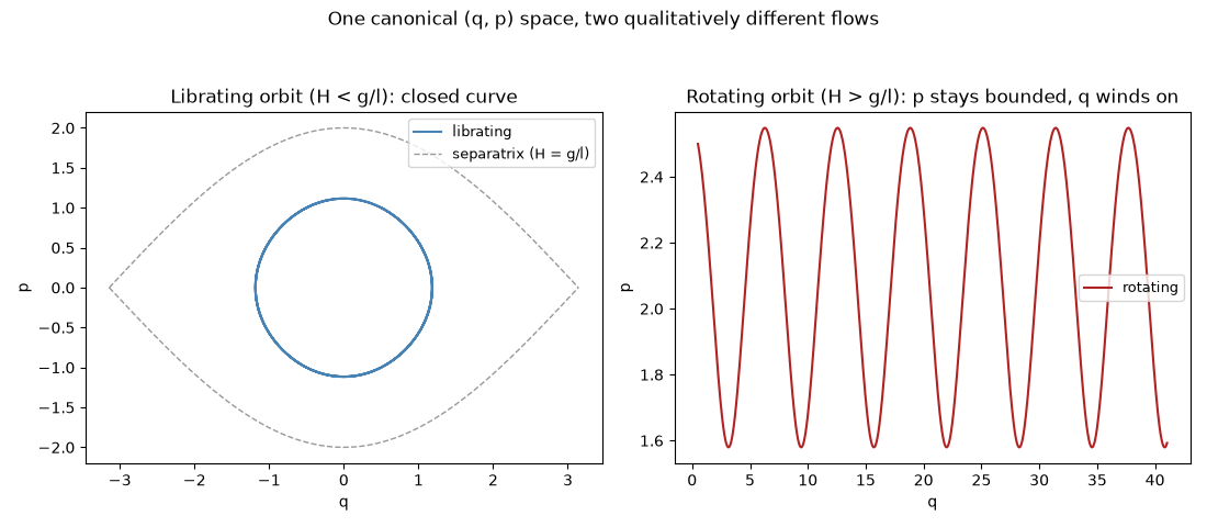
A pendulum below the separatrix (H < g/l) librates; one above it rotates over the top instead. Both are governed by the same H = p^2/2 - (g/l)*cos(q) and the same Hamilton’s equations – only the initial (q, p) point differs.

system = PendulumSwarm(q0=np.array([0.5, 0.5]), p0=np.array([1.0, 2.5]), g_over_l=g_over_l)
H0 = system.per_particle_energy()
result = system.integrate((0.0, 20.0), dt=0.01, method="yoshida4")
H_final = system.per_particle_energy()
print(f"librating pendulum (H = p^2/2 - (g/l)cos(q)): H0={H0[0]:.4f}, H_final={H_final[0]:.4f}")
print(f"rotating pendulum:                            H0={H0[1]:.4f}, H_final={H_final[1]:.4f}")
print(f"separatrix energy g/l = {g_over_l:.4f}")

librating pendulum (H = p^2/2 - (g/l)cos(q)): H0=-0.3776, H_final=-0.3776
rotating pendulum:                            H0=2.2474, H_final=2.2474
separatrix energy g/l = 1.0000

Both trajectories in the unified (q, p) phase space

The librating orbit is a closed loop; the rotating orbit drifts ever further in q while p stays bounded – but both are ordinary curves in the very same (q, p) plane, on either side of the separatrix.

theta = np.linspace(-np.pi, np.pi, 400)
p_separatrix = np.sqrt(np.maximum(2 * g_over_l * (1 + np.cos(theta)), 0))

fig1, axes = plt.subplots(1, 2, figsize=(11, 4.8))
plot_phase_portrait(result.q[:, 0], result.p[:, 0], ax=axes[0], color="steelblue", label="librating")
axes[0].plot(theta, p_separatrix, "0.6", ls="--", lw=1)
axes[0].plot(theta, -p_separatrix, "0.6", ls="--", lw=1, label="separatrix (H = g/l)")
axes[0].set_xlabel("q")
axes[0].set_ylabel("p")
axes[0].set_title("Librating orbit (H < g/l): closed curve")
axes[0].legend(fontsize=9)

plot_phase_portrait(result.q[:, 1], result.p[:, 1], ax=axes[1], color="firebrick", label="rotating")
axes[1].set_xlabel("q")
axes[1].set_ylabel("p")
axes[1].set_title("Rotating orbit (H > g/l): p stays bounded, q winds on")
axes[1].legend(fontsize=9)
fig1.suptitle("One canonical (q, p) space, two qualitatively different flows")
fig1.tight_layout(rect=[0, 0, 1, 0.93])

q(t): bounded oscillation vs. unbounded winding

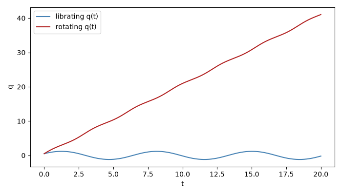
The same qualitative split shows up directly in q(t): the librating pendulum oscillates within fixed bounds forever, while the rotating one’s angle grows without bound as it keeps going over the top.

fig2, ax2 = plt.subplots(figsize=(7, 4))
ax2.plot(result.t, result.q[:, 0], color="steelblue", label="librating q(t)")
ax2.plot(result.t, result.q[:, 1], color="firebrick", label="rotating q(t)")
ax2.set_xlabel("t")
ax2.set_ylabel("q")
ax2.legend()
fig2.tight_layout()

plt.show()