The double pendulum and deterministic chaos

DoublePendulum is two point masses \(m_1, m_2\) on massless rigid rods of length \(l_1, l_2\), the second hanging from the first, with generalized coordinates \(q = (\theta_1, \theta_2)\) measured from the downward vertical:

\[x_1 = l_1\sin\theta_1, \quad y_1 = -l_1\cos\theta_1, \qquad x_2 = x_1 + l_2\sin\theta_2, \quad y_2 = y_1 - l_2\cos\theta_2 .\]

Its Lagrangian \(L = T - V\) is built symbolically from these positions,

\[T = \tfrac12 m_1(\dot x_1^2+\dot y_1^2) + \tfrac12 m_2(\dot x_2^2+\dot y_2^2), \qquad V = m_1 g y_1 + m_2 g y_2 ,\]

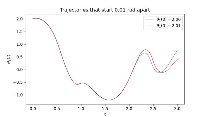
and LagrangianEngine derives the Euler-Lagrange equations of motion, \(\frac{d}{dt}\frac{\partial L}{\partial \dot q_i} - \frac{\partial L}{\partial q_i} = 0\), automatically. Because the resulting mass matrix \(M(\theta_1, \theta_2)\) depends on the configuration (it is not separable), the system is integrated with the general (non-separable-capable) implicit-midpoint symplectic integrator. This example shows that two trajectories launched 0.01 rad apart track each other briefly and then diverge completely: deterministic chaos, not integration error (energy stays conserved throughout; see tests/test_conservation.py).

See SideBySideAnimator: physical space + phase/energy diagnostics, live for an animated side-by-side view of this same system.

import matplotlib.pyplot as plt
import numpy as np

from physicskit.classical.systems.lagrangian import DoublePendulum

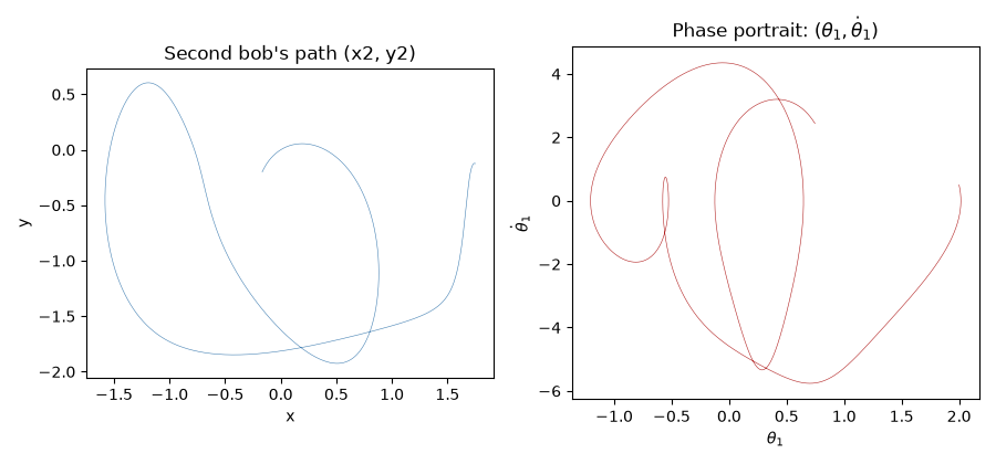
Trajectory and phase portrait

pendulum = DoublePendulum(theta0=[2.0, 1.0], thetadot0=[0.5, -0.3])
result = pendulum.integrate((0, 3.0), dt=3e-5, method="implicit_midpoint")
tip = np.array([pendulum.positions(q) for q in result.q])

fig1, axes = plt.subplots(1, 2, figsize=(9, 4.2))
axes[0].plot(tip[:, 2], tip[:, 3], color="steelblue", lw=0.4)
axes[0].set_title("Second bob's path (x2, y2)")
axes[0].set_aspect("equal")
axes[0].set_xlabel("x")
axes[0].set_ylabel("y")

axes[1].plot(result.q[:, 0], result.p[:, 0], color="firebrick", lw=0.4)
axes[1].set_title(r"Phase portrait: $(\theta_1, \dot\theta_1)$")
axes[1].set_xlabel(r"$\theta_1$")
axes[1].set_ylabel(r"$\dot\theta_1$")
fig1.tight_layout()

Sensitivity to initial conditions

Two trajectories launched a hundredth of a radian apart track each other briefly, then diverge completely – the defining signature of deterministic chaos (first analyzed rigorously for the 3-body problem by Poincare).

p1 = DoublePendulum(theta0=[2.0, 1.0], thetadot0=[0.5, -0.3])
p2 = DoublePendulum(theta0=[2.01, 1.0], thetadot0=[0.5, -0.3])

r1 = p1.integrate((0, 3.0), dt=3e-5, method="implicit_midpoint")
r2 = p2.integrate((0, 3.0), dt=3e-5, method="implicit_midpoint")

drift1 = np.max(np.abs(r1.energy - r1.energy[0])) / abs(r1.energy[0])
print(f"energy drift over 1e5 steps: {drift1:.3e} (chaos below is real dynamics, not numerical error)")

fig2, ax = plt.subplots(figsize=(7, 4))
ax.plot(r1.t, r1.q[:, 0], color="steelblue", lw=0.8, label=r"$\theta_1(0)=2.00$")
ax.plot(r2.t, r2.q[:, 0], color="firebrick", lw=0.8, label=r"$\theta_1(0)=2.01$")
ax.set_xlabel("t")
ax.set_ylabel(r"$\theta_1(t)$")
ax.set_title("Trajectories that start 0.01 rad apart")
ax.legend()

energy drift over 1e5 steps: 1.791e-07 (chaos below is real dynamics, not numerical error)

<matplotlib.legend.Legend object at 0x34dd0d520>

Because implicit_midpoint exactly conserves quadratic invariants of any ODE and is symplectic for canonical Hamiltonians in general, the divergence above is the real chaotic dynamics, not integration error. See also The bead on a rotating hoop: a pitchfork bifurcation and Coupled oscillators: normal modes of a small harmonic chain, built the same symbolic way.

plt.show()