The bead on a rotating hoop: a pitchfork bifurcation

BeadOnRotatingHoop is a bead sliding without friction on a circular hoop of radius \(R\), forced to rotate at fixed angular speed \(\Omega\) about its vertical diameter. With generalized coordinate \(\theta\) (the bead’s polar angle on the hoop), the Lagrangian in the rotating frame is

\[L = \frac{R^2}{2}\left(\dot\theta^2 + \Omega^2\sin^2\theta\right) - g R (1 - \cos\theta) ,\]

which is autonomous, so the dynamics reduce to motion in a 1-DOF effective potential

\[V_\mathrm{eff}(\theta) = g R (1 - \cos\theta) - \frac{1}{2} R^2 \Omega^2 \sin^2\theta .\]

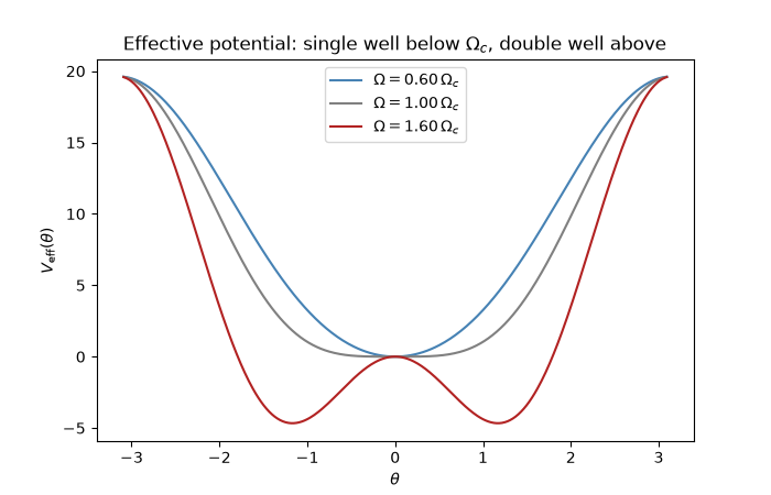
Below the critical rotation speed \(\Omega_c = \sqrt{g/R}\), \(\theta=0\) (the bottom of the hoop) is the bead’s only stable equilibrium. Above it, \(\theta=0\) becomes unstable and two new symmetric stable equilibria appear at \(\cos\theta_\mathrm{eq} = g/(R\Omega^2)\) – a textbook pitchfork bifurcation, visible both in the effective potential’s shape and in where a small perturbation actually settles.

import matplotlib.pyplot as plt
import numpy as np

from physicskit.classical.systems.lagrangian import BeadOnRotatingHoop

R, g = 1.0, 9.81
omega_c = np.sqrt(g / R)
print(f"critical rotation speed: Omega_c = {omega_c:.4f} rad/s")


def v_eff(theta, omega):
    return g * R * (1 - np.cos(theta)) - 0.5 * R**2 * omega**2 * np.sin(theta) ** 2

critical rotation speed: Omega_c = 3.1321 rad/s

Effective potential before/after the bifurcation

theta = np.linspace(-np.pi + 0.05, np.pi - 0.05, 400)

fig1, ax = plt.subplots(figsize=(7, 4.5))
for omega, style in [(0.6 * omega_c, "steelblue"), (omega_c, "0.5"), (1.6 * omega_c, "firebrick")]:
    ax.plot(theta, v_eff(theta, omega), color=style, label=rf"$\Omega = {omega / omega_c:.2f}\,\Omega_c$")
ax.set_xlabel(r"$\theta$")
ax.set_ylabel(r"$V_\mathrm{eff}(\theta)$")
ax.set_title("Effective potential: single well below $\\Omega_c$, double well above")
ax.legend()

<matplotlib.legend.Legend object at 0x16b5c4ad0>

A tiny nudge from theta=0 behaves differently below/above Omega_c

Below Omega_c, theta=0 is the only minimum: the bead oscillates through it, symmetric about zero. Above Omega_c, theta=0 has become a local MAXIMUM separating the two new wells: with essentially zero energy above that local max, the bead is trapped on whichever side it was nudged toward (broken symmetry – it never swings back through theta=0), oscillating within that well between (approximately) its starting point and the mirror point on the well’s far side, with the well’s minimum theta_eq lying inside that range.

below = BeadOnRotatingHoop(theta0=0.05, thetadot0=0.0, R=R, omega=0.6 * omega_c, g=g)
above = BeadOnRotatingHoop(theta0=0.05, thetadot0=0.0, R=R, omega=1.6 * omega_c, g=g)

res_below = below.integrate((0, 20), dt=1e-3, method="implicit_midpoint")
res_above = above.integrate((0, 20), dt=1e-3, method="implicit_midpoint")

theta_eq_above = np.arccos(g / (R * (1.6 * omega_c) ** 2))
theta_above = res_above.q[:, 0]
print(f"predicted new well minimum above Omega_c: theta_eq = {theta_eq_above:.4f} rad")
inside_range = theta_above.min() < theta_eq_above < theta_above.max()
print(f"observed range above Omega_c: [{theta_above.min():.4f}, {theta_above.max():.4f}] rad (theta_eq inside it: {inside_range})")
print(f"stayed on the positive side the whole time (broken symmetry): {bool(np.all(theta_above > -1e-6))}")

fig2, ax2 = plt.subplots(figsize=(7, 4))
ax2.plot(res_below.t, res_below.q[:, 0], color="steelblue", label=r"$\Omega = 0.6\,\Omega_c$ (oscillates through 0)")
ax2.plot(res_above.t, res_above.q[:, 0], color="firebrick", label=r"$\Omega = 1.6\,\Omega_c$ (trapped on one side)")
ax2.axhline(theta_eq_above, color="firebrick", ls="--", lw=0.8, label=r"well minimum $\theta_\mathrm{eq}$")
ax2.axhline(0.0, color="0.6", lw=0.8)
ax2.set_xlabel("t")
ax2.set_ylabel(r"$\theta(t)$")
ax2.set_title("Same tiny initial nudge, broken symmetry above $\\Omega_c$")
ax2.legend()

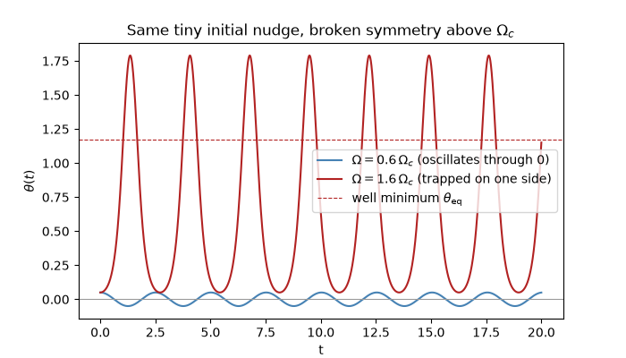
predicted new well minimum above Omega_c: theta_eq = 1.1695 rad
observed range above Omega_c: [0.0500, 1.7900] rad (theta_eq inside it: True)
stayed on the positive side the whole time (broken symmetry): True

<matplotlib.legend.Legend object at 0x34f3482c0>

Like DoublePendulum, this system’s equations of motion are derived symbolically by LagrangianEngine and integrated with implicit_midpoint.

plt.show()