Coupled oscillators: normal modes of a small harmonic chain

CoupledOscillators is a chain of \(N\) masses \(m\) connected in a line by identical linear springs \(k\), both ends fixed to immovable walls – the small-\(N\), exactly-linear prototype for the larger lattice chains in physicskit.classical.systems.chains. With generalized coordinates \(q_i\) (displacement of mass \(i\) from equilibrium) and \(q_0 = q_{N+1} = 0\), the Lagrangian \(L = T - V\) built symbolically by LagrangianEngine is

\[T = \sum_{i=1}^{N} \frac{m}{2}\dot q_i^2, \qquad V = \sum_{i=0}^{N} \frac{k}{2}(q_{i+1} - q_i)^2 ,\]

whose normal modes are the sine waves with closed-form angular frequencies

\[\omega_k = 2\sqrt{\frac{k}{m}} \sin\!\left(\frac{k\pi}{2(N+1)}\right), \qquad k = 1, \dots, N .\]

Exciting a single normal-mode shape keeps every mass oscillating at exactly that mode’s analytic frequency \(\omega_k\) – no mode-mixing, unlike the non-linear FPUTChain (see The Fermi-Pasta-Ulam-Tsingou recurrence) – which this script verifies directly by comparing the simulated period to the closed-form \(\omega_k\) above.

import matplotlib.pyplot as plt
import numpy as np

from physicskit.classical.systems.lagrangian import CoupledOscillators

n, m, k = 4, 1.0, 1.0
mode = 2

# Analytic normal-mode shape and frequency for a fixed-fixed harmonic chain.
sites = np.arange(1, n + 1)
q0 = 0.3 * np.sin(sites * mode * np.pi / (n + 1))
omega_k = 2.0 * np.sqrt(k / m) * np.sin(mode * np.pi / (2.0 * (n + 1)))
period = 2 * np.pi / omega_k
print(f"mode {mode} analytic angular frequency: {omega_k:.4f} rad/s, period: {period:.4f} s")

system = CoupledOscillators(q0, np.zeros(n), n=n, m=m, k=k)
result = system.integrate((0, 3 * period), dt=period / 2000, method="implicit_midpoint")

fig1, ax = plt.subplots(figsize=(8, 4.5))
for i in range(n):
    ax.plot(result.t, result.q[:, i], label=f"mass {i + 1}")
for t_period in np.arange(0, 3 * period, period):
    ax.axvline(t_period, color="0.85", lw=0.8, zorder=0)
ax.set_xlabel("t")
ax.set_ylabel(r"$q_i(t)$")
ax.set_title(f"Pure mode-{mode} excitation: every mass at the same single frequency")
ax.legend(ncol=n)
fig1.tight_layout()

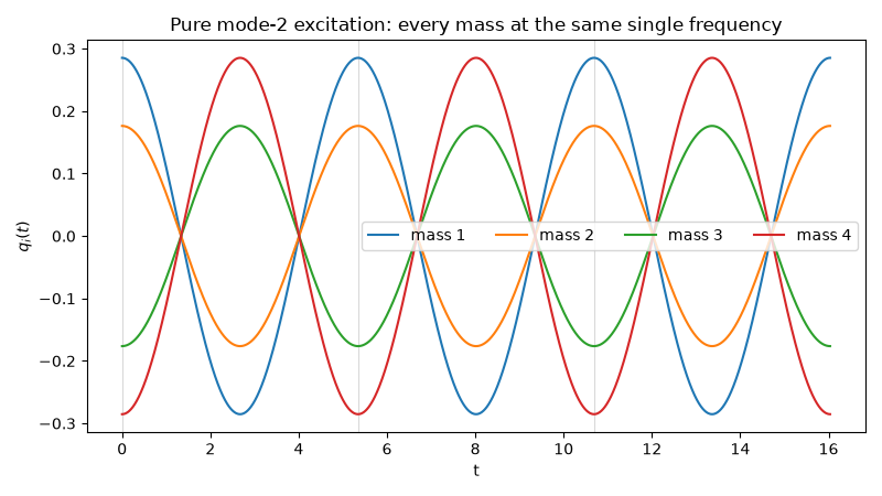
mode 2 analytic angular frequency: 1.1756 rad/s, period: 5.3448 s

Energy conservation and phase portrait for one mass

drift = np.max(np.abs(result.energy - result.energy[0])) / abs(result.energy[0])
print(f"relative energy drift: {drift:.3e}")

fig2, ax2 = plt.subplots(figsize=(6, 5))
ax2.plot(result.q[:, 0], result.p[:, 0], color="steelblue")
ax2.set_xlabel(r"$q_1$")
ax2.set_ylabel(r"$\dot q_1$")
ax2.set_title("Phase portrait of mass 1:\na clean ellipse (single-frequency motion)")
fig2.tight_layout()

plt.show()

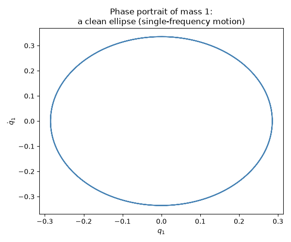
relative energy drift: 3.645e-13