Building your own system: LagrangianEngine from scratch

Every Lagrangian system built into physicskit.classical (DoublePendulum, BeadOnRotatingHoop, CoupledOscillators, HeavySymmetricTop) hides its use of LagrangianEngine inside a system class. This example shows the raw workflow directly, for a system that is not already built in: the elastic (spring) pendulum – a mass \(m\) on a spring of natural length \(l_0\) and stiffness \(k\), free to swing as a pendulum too, so its radial “stretch” and angular “swing” motions are coupled. Using polar-style coordinates \(q = (r, \theta)\) for the pivot-to-mass distance and swing angle,

\[x = r\sin\theta, \qquad y = -r\cos\theta , \qquad L = \frac{m}{2}\left(\dot x^2 + \dot y^2\right) - \frac{k}{2}(r - l_0)^2 - m g y ,\]

LagrangianEngine derives the Euler-Lagrange equations of motion and the Legendre-transformed Hamiltonian purely symbolically from this \(L(q, \dot q)\) – no hand-derived formula or dedicated system class required.

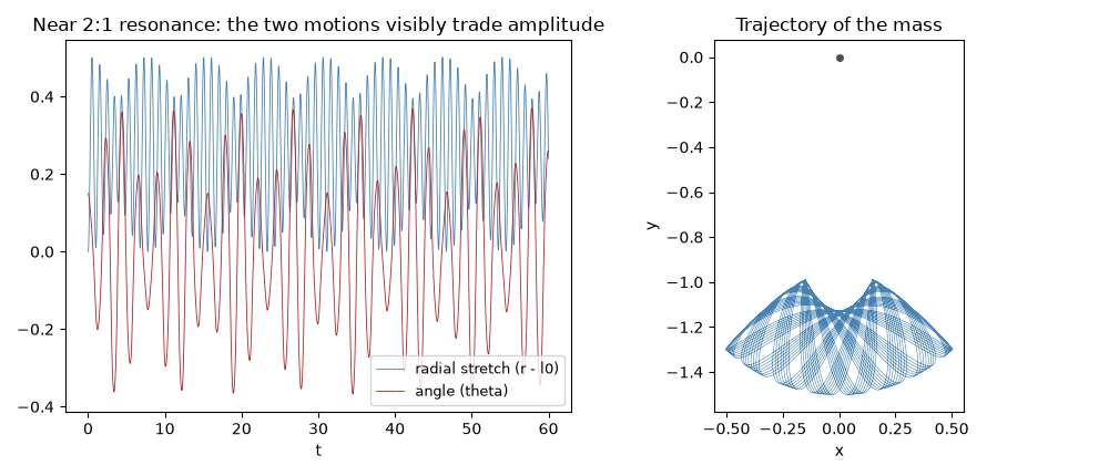
Tuned near the classic 2:1 resonance (spring frequency \(\omega_s = \sqrt{k/m} \approx 2\,\omega_\theta\), twice the pendulum frequency \(\omega_\theta = \sqrt{g/l_0}\)), it shows the textbook energy exchange between the two modes: starting with pure angular swing, energy visibly flows back and forth into radial stretching – not as a single clean beat (the elastic pendulum is famously non-trivial even this close to resonance) but unmistakably present, and still exactly energy-conserving.

import matplotlib.pyplot as plt
import numpy as np
import sympy as sp

from physicskit.classical.core.integrators import implicit_midpoint_integrate
from physicskit.classical.utils.symbolic import LagrangianEngine

Write down L(q, qdot) symbolically

r, theta, rdot, thetadot = sp.symbols("r theta rdot thetadot")
m, k, l0, g = sp.symbols("m k l0 g")

x = r * sp.sin(theta)
y = -r * sp.cos(theta)
xdot = sp.diff(x, r) * rdot + sp.diff(x, theta) * thetadot
ydot = sp.diff(y, r) * rdot + sp.diff(y, theta) * thetadot

T = sp.Rational(1, 2) * m * (xdot**2 + ydot**2)
V = sp.Rational(1, 2) * k * (r - l0) ** 2 + m * g * y
L = sp.simplify(T - V)
print("L(r, theta, rdot, thetadot) =", L)

L(r, theta, rdot, thetadot) = g*m*r*cos(theta) - k*(l0 - r)**2/2 + m*(r**2*thetadot**2 + rdot**2)/2

Hand it to LagrangianEngine: no other code needed

g_val, l0_val, m_val = 9.81, 1.0, 1.0
omega_pendulum = np.sqrt(g_val / l0_val)
k_val = 4 * omega_pendulum**2 * m_val  # the 2:1 resonance condition

engine = LagrangianEngine([r, theta], [rdot, thetadot], L, params={m: m_val, k: k_val, l0: l0_val, g: g_val})
print(f"derived Hamiltonian: {engine.H_expr}")

derived Hamiltonian: 0.5*p0**2 + 0.5*p1**2/r**2 - 9.81*r*cos(theta) + 19.62*(r - 1.0)**2

Integrate directly with the compiled equations of motion

q0 = np.array([l0_val, 0.15])  # spring at rest length, pure angular displacement
qdot0 = np.array([0.0, 0.0])
p0 = engine.momentum_njit(q0, qdot0)
H0 = engine.hamiltonian_njit(q0, p0, 0.0)
y0 = np.concatenate([q0, p0])

n_steps, dt = 60_000, 1e-3
ts, ys = implicit_midpoint_integrate(engine.canonical_deriv_njit, y0, 0.0, n_steps, dt)
r_t, theta_t = ys[:, 0], ys[:, 1]
Hs = np.array([engine.hamiltonian_njit(y[:2], y[2:], 0.0) for y in ys[::50]])
drift = np.max(np.abs(Hs - H0)) / abs(H0)
print(f"energy drift over {n_steps} steps: {drift:.3e}")

fig1, axes = plt.subplots(1, 2, figsize=(10, 4.3))
axes[0].plot(ts, r_t - l0_val, color="steelblue", lw=0.6, label="radial stretch (r - l0)")
axes[0].plot(ts, theta_t, color="firebrick", lw=0.6, label="angle (theta)")
axes[0].set_xlabel("t")
axes[0].set_title("Near 2:1 resonance: the two motions visibly trade amplitude")
axes[0].legend(fontsize=9)

x_t = r_t * np.sin(theta_t)
y_t = -r_t * np.cos(theta_t)
axes[1].plot(x_t, y_t, color="steelblue", lw=0.4)
axes[1].plot(0, 0, "o", color="0.3", ms=4)
axes[1].set_xlabel("x")
axes[1].set_ylabel("y")
axes[1].set_title("Trajectory of the mass")
axes[1].set_aspect("equal")
fig1.tight_layout()

energy drift over 60000 steps: 1.871e-07

The whole workflow is four steps: write q, qdot as SymPy symbols, write down L in terms of them, hand both to LagrangianEngine(q, qdot, L, params=...), and integrate the resulting engine.canonical_deriv_njit – no new system class required.

plt.show()