Noether’s Theorem and the Kepler Problem’s Hidden Symmetry

Emmy Noether’s theorem ties each continuous symmetry of a system’s action to an exactly conserved quantity built from it: time-translation symmetry gives energy, rotational symmetry gives angular momentum. The Kepler problem carries a third, less obvious conserved quantity, the Laplace-Runge-Lenz vector

\[\mathbf{A} = \mathbf{p} \times L - \mu k \hat{\mathbf{r}}, \qquad L = x p_y - y p_x ,\]

fixed in both magnitude and direction only for the exact inverse-square potential – the classical fingerprint of a “hidden,” purely dynamical \(SO(4)\) symmetry, with no equally obvious geometric transformation of space and time behind it the way a rotation or translation is. Any purely radial perturbation to \(V(r) = -k/r\) leaves the manifest rotational symmetry – and hence angular momentum – completely untouched (a central force exerts no torque about its center regardless of its radial profile), while still breaking the hidden symmetry and setting the Laplace-Runge-Lenz vector adrift. Comparing all three conserved quantities’ drift, pure vs. perturbed, makes the distinction concrete: some conservation laws come from symmetries obvious enough to write down by inspection, others do not.

import matplotlib.pyplot as plt
import numpy as np

from physicskit.classical.systems.newtonian import KeplerSystem
from physicskit.classical.utils.conservation import angular_momentum_drift, lrl_drift, relative_energy_drift

Pure vs. perturbed: the same manifest symmetry, a different hidden one

Both systems share exactly the same central-force rotational symmetry; only the perturbed one loses the extra structure special to \(1/r\).

pure = KeplerSystem.from_orbital_elements(a=1.0, e=0.4)
perturbed = KeplerSystem.from_orbital_elements(a=1.0, e=0.4, c_pn=0.01)

res_pure = pure.integrate((0, 200), dt=1e-3, method="yoshida4")
res_pert = perturbed.integrate((0, 200), dt=1e-3, method="yoshida4")

E_pure, E_pert = relative_energy_drift(res_pure.energy), relative_energy_drift(res_pert.energy)
L_pure, L_pert = angular_momentum_drift(res_pure.q, res_pure.p), angular_momentum_drift(res_pert.q, res_pert.p)
A_pure, A_pert = lrl_drift(pure, res_pure.q, res_pure.p), lrl_drift(perturbed, res_pert.q, res_pert.p)

print(f"pure 1/r:  max energy drift={E_pure.max():.2e}, max L drift={L_pure.max():.2e}, max |A| drift={A_pure.max():.2e}")
print(f"perturbed: max energy drift={E_pert.max():.2e}, max L drift={L_pert.max():.2e}, max |A| drift={A_pert.max():.2e}")

fig, axes = plt.subplots(1, 3, figsize=(13, 4.2), sharex=True)
labels = (
    "time-translation\n$\\to$ energy",
    "rotation\n$\\to$ angular momentum",
    "hidden $SO(4)$\n$\\to$ Laplace-Runge-Lenz",
)
for ax, drift_pure, drift_pert, label in zip(axes, (E_pure, L_pure, A_pure), (E_pert, L_pert, A_pert), labels):
    # Each of these drifts is itself oscillatory and periodically crosses
    # exactly zero, so a plain semilogy plot would blow the axis out to
    # 300+ orders of magnitude at every crossing; floor at a fixed noise
    # level (well above float64 round-off, well below the LRL drift this
    # plot exists to show) to keep the comparison legible instead.
    ax.semilogy(res_pure.t, np.maximum(drift_pure, 1e-14), color="steelblue", label="pure 1/r")
    ax.semilogy(res_pert.t, np.maximum(drift_pert, 1e-14), color="firebrick", label="perturbed ($c_{pn} \\neq 0$)")
    ax.set_ylim(1e-14, 1.0)
    ax.set_title(label, fontsize=11)
    ax.set_xlabel("t")
axes[0].set_ylabel("drift from t=0 value")
axes[0].legend(fontsize=8)
fig.suptitle("Only the hidden symmetry's conserved quantity notices the perturbation", fontsize=13)
fig.tight_layout(rect=[0, 0, 1, 0.90])

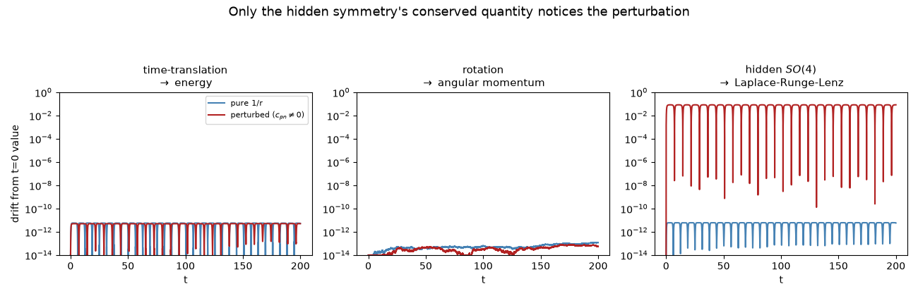
pure 1/r:  max energy drift=5.71e-12, max L drift=1.24e-13, max |A| drift=6.12e-12
perturbed: max energy drift=5.16e-12, max L drift=8.10e-14, max |A| drift=8.36e-02

Energy and angular momentum drift stay pinned at integrator round-off in both columns – time-translation and rotational symmetry are untouched by a purely radial perturbation. Only the Laplace-Runge-Lenz panel tells the two systems apart: flat for the pure potential, growing for the perturbed one, tracking the same perihelion precession visualized directly in Kepler orbits and perihelion precession.

plt.show()