Cuprate Physics: Antiferromagnetism from the Strong-Coupling Hubbard Model

Bednorz and Muller’s 1986 discovery of superconductivity above 30 K in La-Ba-Cu-O launched the search for the cuprate superconductors, whose undoped parent compounds are not metals at all but antiferromagnetic Mott insulators – exactly the strong-coupling (\(U/t \gg 1\)), half-filled regime of the Hubbard model already implemented in hubbard_1d_exact_diagonalization(). No dedicated cuprate (multi-band Emery, or \(t\)-\(J\)) model is implemented here, but the same single-band Hubbard Hamiltonian used for the 1963 Mott-transition example, pushed to half filling and strong coupling, already reproduces the qualitative signature: short-range Neel (antiferromagnetic) spin order, the arena any theory of cuprate pairing has to live in. hubbard_spin_correlations() extracts \(\langle S_i^z S_j^z\rangle\) directly from the many-body ground state, using that \(S^z\) is diagonal in the occupation-number basis the exact-diagonalization solver already works in.

import matplotlib.pyplot as plt
import numpy as np

from physicskit.condensed.correlated import hubbard_1d_exact_diagonalization, hubbard_spin_correlations

Short-range Neel order strengthens with U/t

A half-filled 6-site ring (periodic, so every site is equivalent) at increasing onsite repulsion U: nearest-neighbor spins become more sharply antialigned, and the correlation’s sign alternates with separation – the finite-size fingerprint of antiferromagnetic order, sharpening as double occupancy is suppressed and each site approaches a single, well-defined local moment.

n_sites = 6
U_values = [0.0, 2.0, 8.0, 20.0]
correlations = []
for U in U_values:
    result = hubbard_1d_exact_diagonalization(n_sites=n_sites, n_up=3, n_dn=3, t=1.0, U=U, pbc=True, return_eigenvectors=True)
    corr = hubbard_spin_correlations(n_sites, result["ground_state_vector"], result["states_up"], result["states_dn"])
    correlations.append(corr)
    print(f"U/t = {U:5.1f}: <Sz_0 Sz_0> = {corr[0]:+.4f}, <Sz_0 Sz_1> = {corr[1]:+.4f}, <Sz_0 Sz_2> = {corr[2]:+.4f}")

fig, axes = plt.subplots(1, 2, figsize=(11, 4.3))
r = np.arange(n_sites)
for U, corr in zip(U_values, correlations):
    axes[0].plot(r, corr, "o-", label=f"U/t = {U:g}")
axes[0].axhline(0, color="black", lw=0.5)
axes[0].set_xlabel("separation r")
axes[0].set_ylabel(r"$\langle S_0^z S_r^z \rangle$")
axes[0].set_title("Spin correlations vs. separation")
axes[0].legend(fontsize=8)

nn_correlation = [corr[1] for corr in correlations]
axes[1].plot(U_values, nn_correlation, "o-", color="firebrick")
axes[1].axhline(-0.25, color="black", lw=0.5, ls="--", label="classical Neel limit")
axes[1].set_xlabel("U/t")
axes[1].set_ylabel(r"$\langle S_0^z S_1^z \rangle$ (nearest neighbor)")
axes[1].set_title("Antiferromagnetic correlation strengthens with U/t")
axes[1].legend(fontsize=8)
fig.tight_layout()

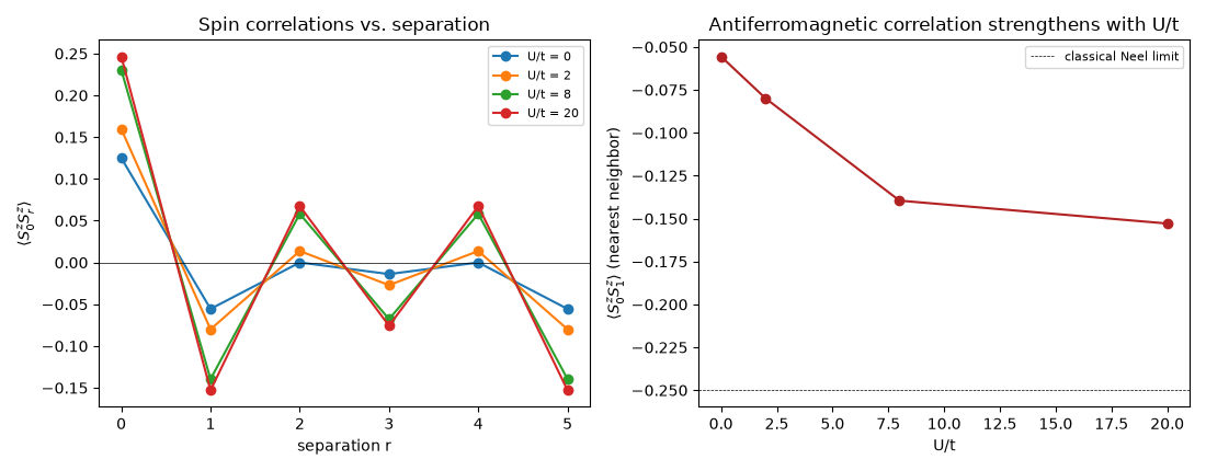
U/t =   0.0: <Sz_0 Sz_0> = +0.1250, <Sz_0 Sz_1> = -0.0556, <Sz_0 Sz_2> = +0.0000
U/t =   2.0: <Sz_0 Sz_0> = +0.1596, <Sz_0 Sz_1> = -0.0800, <Sz_0 Sz_2> = +0.0137
U/t =   8.0: <Sz_0 Sz_0> = +0.2304, <Sz_0 Sz_1> = -0.1395, <Sz_0 Sz_2> = +0.0582
U/t =  20.0: <Sz_0 Sz_0> = +0.2465, <Sz_0 Sz_1> = -0.1529, <Sz_0 Sz_2> = +0.0675

Even on a 6-site ring, far from the thermodynamic-limit cuprate plane, the trend is unambiguous: as U/t grows the ground state is pushed toward the singly-occupied, strong-coupling regime where the effective low-energy physics is a Heisenberg antiferromagnet (the same \(U \to \infty\) limit that gives the \(t\)-\(J\) model widely used as a minimal cuprate Hamiltonian), and nearest-neighbor correlations sharpen toward the classical Neel value of \(-1/4\).

plt.show()