Graphene: A Massless Dirac Cone on a Honeycomb Lattice

Geim and Novoselov’s isolation of a single atomic layer of graphite produced the first genuinely 2D crystal – and its low-energy quasiparticles obey a massless relativistic (Dirac) equation rather than the ordinary Schrodinger equation, turning a tabletop material into a laboratory for relativistic quantum phenomena. graphene_hamiltonian() reproduces this linear dispersion near the honeycomb lattice’s Brillouin zone corners.

import matplotlib.pyplot as plt
import numpy as np

from physicskit.condensed.models import graphene_hamiltonian

Sampling H(k) through the Dirac point

The two inequivalent Brillouin-zone corners \(K=(2\pi/3, 4\pi/3)\) and \(K'\) are where the honeycomb lattice’s two sublattice bands touch. Scanning a line of momenta through \(K\) shows the gap close exactly at the center and the bands disperse linearly on either side.

K = np.array([2 * np.pi / 3, 4 * np.pi / 3])
q = np.linspace(-0.3, 0.3, 201)
bands = np.array([np.linalg.eigvalsh(graphene_hamiltonian(*(K + [dq, 0]))) for dq in q])

fig, ax = plt.subplots(figsize=(6, 4))
ax.plot(q, bands, color="C0")
ax.axvline(0, color="gray", ls="--")
ax.set_xlabel(r"$q$ (distance from Dirac point $K$)")
ax.set_ylabel("Energy")
ax.set_title(r"Massless Dirac cone: $E(q) \sim \pm v_F|q|$")
fig.tight_layout()

gap_at_K = bands[len(q) // 2, 1] - bands[len(q) // 2, 0]
slope = (bands[-1, 1] - bands[len(q) // 2, 1]) / (q[-1] - q[len(q) // 2])
print(f"gap exactly at K: {gap_at_K:.2e} (closes)")
print(f"local slope dE/dq away from K: {slope:.4f} (linear, not quadratic)")

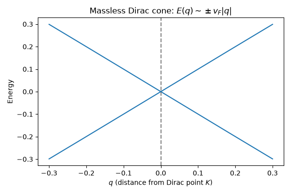
gap exactly at K: 8.01e-16 (closes)
local slope dE/dq away from K: 0.9963 (linear, not quadratic)