Graphene: Zero-Energy Edge States on a Zigzag-Terminated Flake

Graphene: A Massless Dirac Cone on a Honeycomb Lattice looks at graphene’s bulk Bloch spectrum – a linear Dirac cone with no gap. Cutting a finite flake out of the honeycomb lattice along its two primitive-lattice directions produces the classic “zigzag” edge termination, and with it a macroscopically degenerate band of zero-energy states with no bulk counterpart, localized entirely on the flake’s boundary and almost entirely on a single sublattice. Unlike the SSH or Haldane edge states elsewhere in this gallery, these zero modes are not protected by a bulk topological invariant – they are a purely geometric consequence of the zigzag edge cut, and vanish under an armchair termination instead.

graphene_lattice_hamiltonian() builds the nearest-neighbor honeycomb model on sublattices A and B with hopping amplitude \(t\) and no onsite energy on either sublattice, whose Bloch Hamiltonian (see physicskit.condensed.tight_binding for the reduced-momentum convention) is purely off-diagonal between sublattices,

\[\begin{split}H(k_1, k_2) = \begin{pmatrix} 0 & f(k_1, k_2) \\ f(k_1, k_2)^* & 0 \end{pmatrix}, \qquad f(k_1, k_2) = t\left(1 + e^{-ik_1} + e^{-ik_2}\right).\end{split}\]

Having no diagonal part at all is exactly the chiral (sublattice) symmetry \(\Sigma_z H \Sigma_z = -H\), with \(\Sigma_z = \mathrm{diag}(+1, -1)\) on (A, B): every eigenstate at energy \(E\) pairs with a chiral partner at \(-E\), except for any surplus of sites on one sublattice, which is forced to sit at exactly \(E=0\). This is the same symmetry that pins the SSH chain’s edge modes (The SSH Model: Zak Phase and Protected Edge States); on a bulk (translationally invariant) flake the two sublattices balance exactly, but a zigzag-terminated boundary locally strips sites from one sublattice at each edge, creating the local sublattice imbalance that the zero-energy band lives on. build_finite_cluster() builds the finite, fully open flake directly from this same real-space model.

import matplotlib.pyplot as plt
import numpy as np

from physicskit.condensed.models import graphene_lattice_hamiltonian
from physicskit.condensed.tight_binding import build_finite_cluster
from physicskit.condensed.visualizers import plot_lattice_structure

Building the flake

A rectangular grid of unit cells in the honeycomb lattice’s own primitive directions – rather than a rectangle in Cartesian space – is exactly the standard zigzag-edge construction: cutting along the primitive vectors of the A/B honeycomb basis exposes zigzag edges on all four sides of the resulting parallelogram.

n_cells = 10
H, positions, bonds = build_finite_cluster(graphene_lattice_hamiltonian(t=1.0), n_cells=(n_cells, n_cells))
print(f"flake: {H.shape[0]} sites, {len(bonds)} nearest-neighbor bonds")

flake: 200 sites, 280 nearest-neighbor bonds

The zero-energy edge band

The finite-size spectrum splits into dispersive bulk-like bands and a cluster of states pinned near zero energy, with a level spacing among themselves that shrinks as the flake grows (unlike the bulk gap, which stays open) – the hallmark of a boundary-localized band rather than a single discrete state. Chiral symmetry is what pins this cluster to \(E=0\) rather than merely near it; boundary sites with fewer than the bulk’s three nearest neighbors – the degree < 3 sites identified below – are exactly where the zigzag cut creates the local sublattice imbalance the zero modes live on, so the boundary-density weight computed next is a direct check of that mechanism.

eigenvalues, eigenvectors = np.linalg.eigh(H)
edge_idx = np.where(np.abs(eigenvalues) < 0.2)[0]
print(f"{len(edge_idx)} states pinned near zero energy (|E| < 0.2), out of {H.shape[0]} total")

edge_density = np.sum(np.abs(eigenvectors[:, edge_idx]) ** 2, axis=1)

degree = np.zeros(H.shape[0])
for i, j, _ in bonds:
    degree[i] += 1
    degree[j] += 1
boundary = degree < 3
boundary_fraction = edge_density[boundary].sum() / edge_density.sum()
print(f"boundary sites ({boundary.sum()}/{H.shape[0]}) carry {boundary_fraction:.1%} of the zero-band's weight")

fig, (ax1, ax2) = plt.subplots(1, 2, figsize=(11, 4.5))

ax1.plot(np.arange(H.shape[0]), eigenvalues, ".", color="C0")
ax1.plot(edge_idx, eigenvalues[edge_idx], ".", color="C1", label="near-zero band")
ax1.axhline(0.0, color="gray", ls="--", lw=0.5)
ax1.set_xlabel("Eigenvalue index")
ax1.set_ylabel("Energy")
ax1.set_title("Finite-flake spectrum")
ax1.legend()

plot_lattice_structure(positions, bonds, weights=edge_density, ax=ax2)
ax2.set_title("Zero-energy band density")

fig.suptitle("Graphene zigzag flake: boundary-localized zero-energy states")
fig.tight_layout()

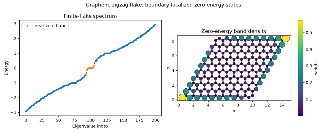
12 states pinned near zero energy (|E| < 0.2), out of 200 total
boundary sites (38/200) carry 73.6% of the zero-band's weight