The Hanbury Brown-Twiss effect: bunching, coherent, and antibunched light

Hanbury Brown and Twiss measured intensity correlations between two separated detectors and found bunching in thermal starlight – the second-order correlation function

\[g^{(2)}(0) = \frac{\langle n(n-1)\rangle}{\langle n\rangle^2}\]

came out at 2 for their chaotic (thermal) source, rather than the value 1 a classical coherent wave gives. This example computes \(g^{(2)}(0)\) directly from photon-number distributions for three cases: a thermal (chaotic) source, built directly from its geometric number distribution; a coherent state, from coherent_state(); and a Fock state, from fock_state() – recovering the historical bunched (2), classical boundary (1), and antibunched (<1) values in one place, and showing where Kimble, Dagenais, and Mandel’s 1977 sub-Poissonian measurement sits relative to Hanbury Brown and Twiss’s own bunched result.

import matplotlib.pyplot as plt
import numpy as np

from physicskit.optics.quantum_optics import coherent_state, fock_state

g^(2)(0) from a photon-number distribution

For any (mixed or pure) photon-number distribution P(n), the zero-delay second-order correlation is exactly the ratio of the second factorial moment to the mean squared – no field amplitudes or detector geometry are needed, only the number statistics.

n_max = 60
n = np.arange(n_max)


def g2_from_distribution(P_n):
    mean_n = np.sum(n * P_n)
    mean_n_nm1 = np.sum(n * (n - 1) * P_n)
    return mean_n_nm1 / mean_n**2

Thermal (chaotic) light: Hanbury Brown and Twiss’s actual source

Thermal light has no single quantum state – it is a statistical mixture with the geometric (Bose-Einstein) number distribution P(n) = nbar^n / (1+nbar)^(n+1). Built directly here, exactly the classical-statistics picture that explained the bunching HBT measured.

n_bar = 3.0
P_thermal = n_bar**n / (1.0 + n_bar) ** (n + 1)
P_thermal /= P_thermal.sum()  # renormalize for the finite truncation
g2_thermal = g2_from_distribution(P_thermal)

Coherent light: the classical Poissonian boundary

alpha = np.sqrt(n_bar)
psi_coherent = coherent_state(alpha, n_max)
P_coherent = np.abs(psi_coherent) ** 2
g2_coherent = g2_from_distribution(P_coherent)

A Fock state: fully antibunched (Kimble, Dagenais, and Mandel’s regime)

k = 3
psi_fock = fock_state(k, n_max)
P_fock = np.abs(psi_fock) ** 2
g2_fock = g2_from_distribution(P_fock)

print(f"thermal (n_bar={n_bar}):   g2(0) = {g2_thermal:.4f}  (Hanbury Brown-Twiss found 2 -- bunched)")
print(f"coherent (<n>={n_bar}):    g2(0) = {g2_coherent:.4f}  (the classical boundary -- neither bunched nor antibunched)")
print(f"Fock |{k}>:              g2(0) = {g2_fock:.4f}  (Kimble-Dagenais-Mandel's regime -- antibunched, no classical field can do this)")

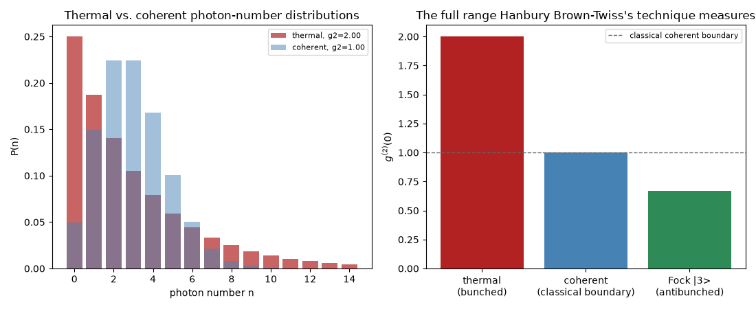
thermal (n_bar=3.0):   g2(0) = 2.0000  (Hanbury Brown-Twiss found 2 -- bunched)
coherent (<n>=3.0):    g2(0) = 1.0000  (the classical boundary -- neither bunched nor antibunched)
Fock |3>:              g2(0) = 0.6667  (Kimble-Dagenais-Mandel's regime -- antibunched, no classical field can do this)

All three, side by side

fig, (ax1, ax2) = plt.subplots(1, 2, figsize=(11, 4.5))
width = 0.8
ax1.bar(n[:15], P_thermal[:15], width, alpha=0.7, label=f"thermal, g2={g2_thermal:.2f}", color="firebrick")
ax1.bar(n[:15], P_coherent[:15], width, alpha=0.5, label=f"coherent, g2={g2_coherent:.2f}", color="steelblue")
ax1.set_xlabel("photon number n")
ax1.set_ylabel("P(n)")
ax1.set_title("Thermal vs. coherent photon-number distributions")
ax1.legend(fontsize=8)

labels = ["thermal\n(bunched)", "coherent\n(classical boundary)", f"Fock |{k}>\n(antibunched)"]
values = [g2_thermal, g2_coherent, g2_fock]
colors = ["firebrick", "steelblue", "seagreen"]
ax2.bar(labels, values, color=colors)
ax2.axhline(1.0, color="0.4", ls="--", lw=1, label="classical coherent boundary")
ax2.set_ylabel(r"$g^{(2)}(0)$")
ax2.set_title("The full range Hanbury Brown-Twiss's technique measures")
ax2.legend(fontsize=8)
fig.tight_layout()

plt.show()