The Jaynes-Cummings model: vacuum Rabi oscillation and collapse-and-revival

Edwin Jaynes and Fred Cummings introduced the minimal fully quantum model of light-matter interaction: a single two-level atom coupled to a single quantized cavity mode. In the rotating-wave approximation, the Hamiltonian JaynesCummingsModel builds is

\[\hat H = \omega_c\, \hat a^\dagger \hat a \otimes \hat I + \frac{\omega_a}{2}\, \hat I \otimes \hat\sigma_z + g\left(\hat a \otimes \hat\sigma_+ + \hat a^\dagger \otimes \hat\sigma_-\right),\]

with cavity frequency \(\omega_c\), atomic transition frequency \(\omega_a\), and atom-cavity coupling strength \(g\). On resonance (\(\omega_c=\omega_a\)), even with the atom initially excited and the field in vacuum, the excited-state population \(P_e(t) = \sum_n|\langle e,n|\psi(t)\rangle|^2\) oscillates coherently at the vacuum Rabi frequency \(2g\) – a phenomenon with no semiclassical counterpart – and for a field prepared in a Fock or coherent state, the oscillations periodically collapse and then revive, direct evidence of the discreteness of the photon number. excited_state_population() reproduces both effects directly.

import matplotlib.pyplot as plt
import numpy as np

from physicskit.optics.quantum_optics import JaynesCummingsModel, coherent_state

Vacuum Rabi oscillation vs. collapse-and-revival with a coherent-state field

A single-Fock-number field gives a single vacuum-Rabi frequency \(2g\sqrt{n+1}\) and oscillates undamped forever; genuine collapse-and-revival requires a field with a spread of photon numbers, each contributing its own Rabi frequency, so that they first dephase (collapse) and later rephase (revive). A coherent state supplies exactly that Poissonian spread, so it is built directly as the initial field and evolved with evolve().

g = 0.5
jc_vacuum = JaynesCummingsModel(omega_c=1.0, omega_a=1.0, g=g, cutoff=10)

cutoff = 60
nbar = 20.0
jc_coherent = JaynesCummingsModel(omega_c=1.0, omega_a=1.0, g=g, cutoff=cutoff)
field = coherent_state(np.sqrt(nbar), cutoff)

# atom excited (flat index 2*n), field in a coherent state -- basis ordering
# documented on JaynesCummingsModel.hamiltonian
psi0 = np.zeros(2 * cutoff, dtype=complex)
psi0[0::2] = field

t_revival = 2 * np.pi * np.sqrt(nbar) / g
t = np.linspace(0, 2.2 * t_revival, 2000)

Pe_vacuum = jc_vacuum.excited_state_population(np.linspace(0, 40, 800), n_photons=0)
psi_t = jc_coherent.evolve(psi0, t)
Pe_coherent = np.sum(np.abs(psi_t[:, 0::2]) ** 2, axis=1).real

On resonance with the field in vacuum, the excited-state population follows the textbook cos^2(g t) formula exactly. With the field instead prepared in a coherent state of mean photon number nbar, the many component Rabi frequencies dephase into a near-featureless collapse and then rephase into a revival near \(t \approx 2\pi\sqrt{\bar n}/g\).

fig, axes = plt.subplots(1, 2, figsize=(11, 4))
axes[0].plot(np.linspace(0, 40, 800), Pe_vacuum)
axes[0].set_xlabel("g t")
axes[0].set_ylabel(r"$P_e(t)$")
axes[0].set_title("n=0: pure vacuum Rabi oscillation")

axes[1].plot(t, Pe_coherent)
axes[1].axvline(t_revival, color="r", ls="--", label=f"predicted revival t={t_revival:.1f}")
axes[1].set_xlabel("t")
axes[1].set_ylabel(r"$P_e(t)$")
axes[1].set_title(f"Coherent field, nbar={nbar:.0f}: collapse & revival")
axes[1].legend(fontsize=8)
fig.tight_layout()

Pe_analytic = np.cos(g * np.linspace(0, 40, 800)) ** 2
max_err = np.max(np.abs(Pe_vacuum - Pe_analytic))
print(f"g = {g}: max |P_e(t) - cos^2(g t)| for n=0 = {max_err:.2e} (textbook vacuum Rabi formula)")

collapse_region = (t > 5) & (t < 12)
revival_region = (t > t_revival - 5) & (t < t_revival + 5)
print(f"coherent-field nbar={nbar:.0f}: predicted revival time = {t_revival:.2f}")
print(f"P_e(t) range during collapse (t in [5,12]):        {Pe_coherent[collapse_region].min():.3f} to {Pe_coherent[collapse_region].max():.3f}")
print(f"P_e(t) range near predicted revival (t~{t_revival:.0f}): {Pe_coherent[revival_region].min():.3f} to {Pe_coherent[revival_region].max():.3f}")
print("the collapsed oscillation's near-flat, reduced amplitude, followed by")
print("a revival of large-amplitude oscillation, is the discreteness-of-")
print("photon-number signature Jaynes and Cummings predicted -- absent from")
print("any semiclassical (classical-field) treatment.")

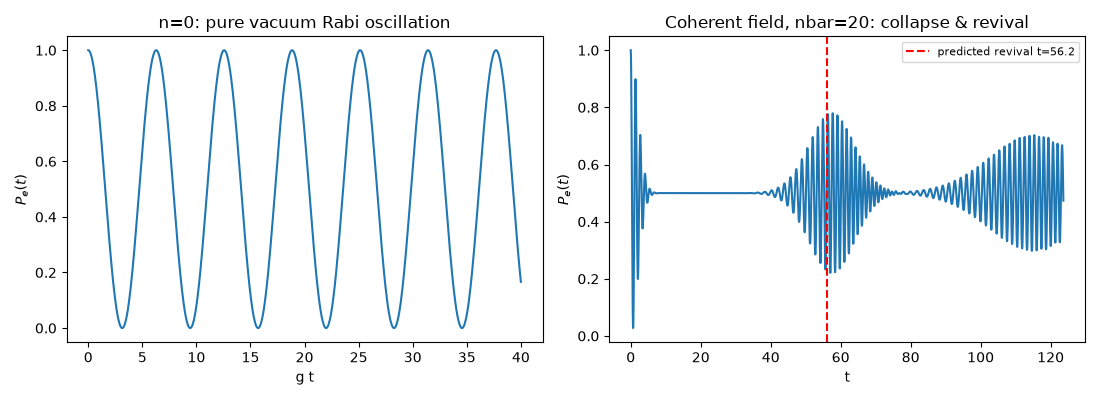
g = 0.5: max |P_e(t) - cos^2(g t)| for n=0 = 8.88e-16 (textbook vacuum Rabi formula)
coherent-field nbar=20: predicted revival time = 56.20
P_e(t) range during collapse (t in [5,12]):        0.488 to 0.515
P_e(t) range near predicted revival (t~56): 0.221 to 0.779
the collapsed oscillation's near-flat, reduced amplitude, followed by
a revival of large-amplitude oscillation, is the discreteness-of-
photon-number signature Jaynes and Cummings predicted -- absent from
any semiclassical (classical-field) treatment.

What is actually collapsing and reviving: the cavity photon-number distribution

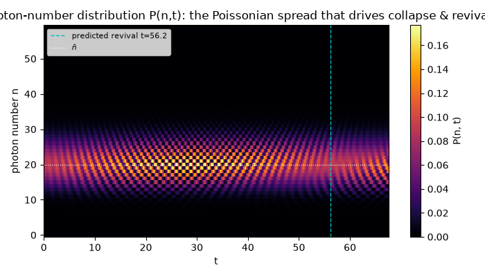
The single P_e(t) curve above is only the atomic projection of a much richer object: the full cavity photon-number probability \(P(n,t) = |\langle e,n|\psi(t)\rangle|^2 + |\langle g,n|\psi(t)\rangle|^2\), already fully contained in the same state psi_t returned by evolve() (basis ordering: flat index 2*n is \(|e,n\rangle\), 2*n+1 is \(|g,n\rangle\)). Plotting it as a 2D image over \((n, t)\) shows probability sloshing coherently between neighboring photon numbers during the collapse, then reorganizing into the revived oscillation.

t_dense = np.linspace(0, 1.2 * t_revival, 400)
psi_t_dense = jc_coherent.evolve(psi0, t_dense)
P_n_t = np.abs(psi_t_dense[:, 0::2]) ** 2 + np.abs(psi_t_dense[:, 1::2]) ** 2  # shape (T, cutoff)

fig2, ax2 = plt.subplots(figsize=(7, 4))
im = ax2.pcolormesh(t_dense, np.arange(cutoff), P_n_t.T, shading="auto", cmap="inferno")
fig2.colorbar(im, ax=ax2, label="P(n, t)")
ax2.axvline(t_revival, color="c", ls="--", lw=1, label=f"predicted revival t={t_revival:.1f}")
ax2.axhline(nbar, color="w", ls=":", lw=0.8, label=r"$\bar n$")
ax2.set_xlabel("t")
ax2.set_ylabel("photon number n")
ax2.legend(fontsize=8)
ax2.set_title("Cavity photon-number distribution P(n,t): the Poissonian spread that drives collapse & revival")
fig2.tight_layout()