Kimble, Dagenais, and Mandel: photon antibunching and the Fano factor

Kimble, Dagenais, and Mandel measured the first direct evidence that light can arrive one photon at a time, with a vanishing probability of detecting two photons simultaneously – no classical wave, however dim, can produce sub-Poissonian photon statistics. The Fano factor \(F = \mathrm{Var}(\hat n)/\langle\hat n\rangle\) equals 1 for a Poissonian (coherent, classical-limit) source and 0 for a number (Fock) state – the fully antibunched, sub-Poissonian extreme their photon-counting statistics approached. fock_state() and coherent_state() give the two limiting photon-number distributions directly, from which the Fano factor is computed as an ordinary first/second moment.

import matplotlib.pyplot as plt
import numpy as np

from physicskit.optics.quantum_optics import coherent_state, compute_wigner_function, fock_state

Fock \(|3\rangle\) (fully antibunched) vs. a coherent state of the same mean photon number

cutoff = 20
n = np.arange(cutoff)


def fano_factor(psi):
    p = np.abs(psi) ** 2
    mean_n = np.sum(n * p)
    var_n = np.sum(n**2 * p) - mean_n**2
    return var_n / mean_n, p


F_fock, P_fock = fano_factor(fock_state(3, cutoff))
F_coh, P_coh = fano_factor(coherent_state(np.sqrt(3.0), cutoff))

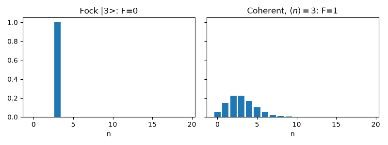
A number state has zero photon-number variance (F=0, fully antibunched: two photons never arrive together), while a coherent state of the same mean photon number is Poissonian (F=1) – the classical boundary that Kimble, Dagenais, and Mandel’s measurement fell decisively below.

fig, axes = plt.subplots(1, 2, figsize=(8, 3), sharey=True)
axes[0].bar(n, P_fock)
axes[0].set_title("Fock |3>: F=0")
axes[0].set_xlabel("n")
axes[1].bar(n, P_coh)
axes[1].set_title(r"Coherent, $\langle n\rangle=3$: F=1")
axes[1].set_xlabel("n")
fig.tight_layout()

print(f"Fock |3>:        Fano factor = {F_fock:.3f}  (fully antibunched, sub-Poissonian)")
print(f"Coherent <n>=3:  Fano factor = {F_coh:.3f}  (classical Poissonian boundary)")
print("no classical field, however attenuated, can produce F < 1: only the")
print("discreteness of the quantized field (the Fock-state extreme) allows it.")

Fock |3>:        Fano factor = 0.000  (fully antibunched, sub-Poissonian)
Coherent <n>=3:  Fano factor = 1.000  (classical Poissonian boundary)
no classical field, however attenuated, can produce F < 1: only the
discreteness of the quantized field (the Fock-state extreme) allows it.

The same two states in phase space: a ring vs. a displaced blob

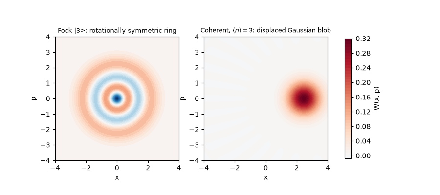
A photon-number bar chart hides where the two states sit in phase space. compute_wigner_function() shows the qualitative difference directly: the fully antibunched Fock state \(|3\rangle\) has no well-defined phase and is rotationally symmetric – a ring in \((x,p)\) – while the coherent state of the same mean photon number is a single Gaussian blob displaced from the origin, the “most classical” phase-space shape available to a quantum state.

x = np.linspace(-4, 4, 121)
p = np.linspace(-4, 4, 121)
W_fock = compute_wigner_function(fock_state(3, cutoff), x, p)
W_coh = compute_wigner_function(coherent_state(np.sqrt(3.0), cutoff), x, p)

fig2, axes2 = plt.subplots(1, 2, figsize=(9, 4))
vmax = max(np.abs(W_fock).max(), np.abs(W_coh).max())
for ax, W, title in zip(axes2, [W_fock, W_coh], ["Fock |3>: rotationally symmetric ring", r"Coherent, $\langle n\rangle=3$: displaced Gaussian blob"]):
    im = ax.contourf(x, p, W.T, levels=40, cmap="RdBu_r", vmin=-vmax, vmax=vmax)
    ax.set_title(title, fontsize=9)
    ax.set_xlabel("x")
    ax.set_ylabel("p")
    ax.set_aspect("equal")
fig2.colorbar(im, ax=axes2, label="W(x, p)", shrink=0.8)

<matplotlib.colorbar.Colorbar object at 0x34d9d0590>