Slusher et al.: squeezed light and sub-vacuum quadrature noise

Richard Slusher and coworkers produced the first experimentally observed squeezed state of light. In terms of the dimensionless field quadratures \(\hat x = (\hat a+\hat a^\dagger)/\sqrt2\) and \(\hat p = (\hat a-\hat a^\dagger)/(i\sqrt2)\), a coherent state divides the quantum uncertainty of the electromagnetic field equally between the two conjugate quadratures; a squeezed state redistributes that uncertainty unequally, reducing the noise in one quadrature below the vacuum (shot-noise) variance of \(1/2\) at the unavoidable cost of increasing it in the other, while the uncertainty product itself remains bounded below. squeezed_state() constructs the squeeze-then-displace state

\[\lvert\xi,\alpha\rangle = \hat D(\alpha)\,\hat S(\xi)\,\lvert 0\rangle, \qquad \hat S(\xi) = \exp\!\left[\frac{\xi^* \hat a^2 - \xi \hat a^{\dagger 2}}{2}\right], \qquad \hat D(\alpha) = \exp\!\left(\alpha \hat a^\dagger - \alpha^* \hat a\right),\]

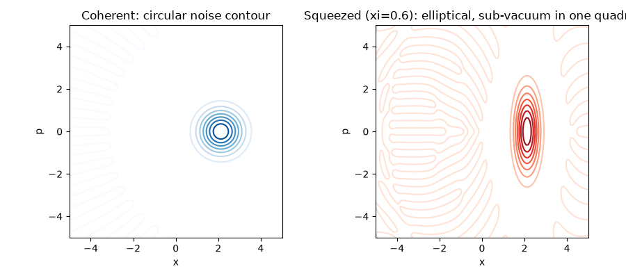
from a squeezing parameter \(\xi = re^{i\theta}\) and displacement \(\alpha\); a real, positive \(\xi\) squeezes the \(p\) quadrature variance down by a factor \(e^{-2r}\) (and stretches \(x\) by \(e^{2r}\)). Its quadrature-asymmetric, sub-vacuum noise character is directly visible in the elliptical, non-circular contours produced by compute_wigner_function() when applied to its state vector, in contrast with a coherent state’s circular contours of equal width in both quadratures.

import matplotlib.pyplot as plt
import numpy as np

from physicskit.optics.quantum_optics import coherent_state, compute_wigner_function, squeezed_state

A squeezed state vs. a coherent state of the same displacement

cutoff = 30
xi = 0.6  # squeezing parameter (real -> squeezes the p quadrature)
psi_coh = coherent_state(1.5, cutoff)
psi_sq = squeezed_state(xi, alpha=1.5, cutoff=cutoff)

x = np.linspace(-5, 5, 121)
p = np.linspace(-5, 5, 121)
W_coh = compute_wigner_function(psi_coh, x, p)
W_sq = compute_wigner_function(psi_sq, x, p)

The coherent state’s noise contour is a circle (equal uncertainty in both quadratures); the squeezed state’s is an ellipse, narrower along one quadrature than the vacuum limit and correspondingly wider along the other.

fig, axes = plt.subplots(1, 2, figsize=(9, 4))
axes[0].contour(x, p, W_coh.T, levels=8, cmap="Blues")
axes[0].set_title("Coherent: circular noise contour")
axes[1].contour(x, p, W_sq.T, levels=8, cmap="Reds")
axes[1].set_title(f"Squeezed (xi={xi}): elliptical, sub-vacuum in one quadrature")
for ax in axes:
    ax.set_xlabel("x")
    ax.set_ylabel("p")
    ax.set_aspect("equal")
fig.tight_layout()


def variance_x(W, x_grid, p_grid):
    marginal = np.trapezoid(W, p_grid, axis=1)
    marginal /= np.trapezoid(marginal, x_grid)
    mean = np.trapezoid(x_grid * marginal, x_grid)
    return np.trapezoid((x_grid - mean) ** 2 * marginal, x_grid)


var_x_vacuum = 0.5  # shot-noise (vacuum) level in these dimensionless quadratures
var_x_squeezed = variance_x(W_sq, x, p)
print(f"vacuum (shot-noise) x-quadrature variance: {var_x_vacuum}")
print(f"squeezed-state x-quadrature variance:      {var_x_squeezed:.4f}")
print(f"predicted e^(-2*xi) reduction: {var_x_vacuum * np.exp(-2 * xi):.4f}")
print("noise pushed below the vacuum level in one quadrature is exactly the")
print("effect Slusher and coworkers first observed experimentally in 1985.")

vacuum (shot-noise) x-quadrature variance: 0.5
squeezed-state x-quadrature variance:      0.1506
predicted e^(-2*xi) reduction: 0.1506
noise pushed below the vacuum level in one quadrature is exactly the
effect Slusher and coworkers first observed experimentally in 1985.