Compton scattering: the photon as a relativistic particle

X-rays scattered off light elements came back with a wavelength shift depending only on the scattering angle – a result the classical wave picture of light could not explain. Compton (1923) treated the X-ray as a genuine relativistic particle, a photon of energy \(E=h\nu\) and momentum \(p=h\nu/c\), colliding elastically with a free electron and imposing ordinary four-momentum conservation on the two-body collision \(\gamma+e^-\to\gamma'+e^{-\prime}\). This example does not assume the textbook formula at all: it solves the conservation equations directly with FourVector arithmetic and a numerical root-find for the outgoing photon energy, then checks the result against the closed-form Compton formula.

import matplotlib.pyplot as plt
import numpy as np
from scipy.optimize import brentq

from physicskit.particle.kinematics import FourVector

Solving four-momentum conservation directly, from scratch

No Compton formula is assumed here: given an incident photon energy E and a scattering angle theta, the outgoing electron’s four-momentum is fixed by conservation once the outgoing photon’s energy E_prime is chosen – electron_mass_residual() returns how far that implied electron is from being on-shell (mass exactly m_e), and scipy.optimize.brentq() finds the E_prime that makes it exactly on-shell, the physically realized solution.

m_e = 0.511  # MeV


def electron_mass_residual(E_prime, E, theta, m_e):
    total = FourVector(E + m_e, 0.0, 0.0, E)  # incident photon (along z) + electron at rest
    photon_out = FourVector(E_prime, E_prime * np.sin(theta), 0.0, E_prime * np.cos(theta))
    electron_out = total - photon_out
    return electron_out.mass - m_e


def solve_outgoing_photon_energy(E, theta):
    return brentq(electron_mass_residual, 1e-9, E, args=(E, theta, m_e))

Checking the result against the closed-form Compton formula

The textbook result, \(\lambda'-\lambda=(1/m_e)(1-\cos\theta)\) (natural units, \(\hbar=c=1\)), translates directly to an energy form via \(E=1/\lambda\):

E_incident = 0.1  # MeV, a typical hard-X-ray/soft-gamma-ray energy
theta_values = np.linspace(0.01, np.pi - 0.01, 60)

E_numeric = np.array([solve_outgoing_photon_energy(E_incident, th) for th in theta_values])
E_formula = E_incident / (1.0 + (E_incident / m_e) * (1.0 - np.cos(theta_values)))

print(f"incident photon energy: {E_incident} MeV")
print(f"max |numeric - formula| across all angles: {np.max(np.abs(E_numeric - E_formula)):.2e} MeV")
print(f"at theta=180 deg (backscatter): E' numeric = {E_numeric[-1]:.6f} MeV, formula = {E_formula[-1]:.6f} MeV")

fig, (ax1, ax2) = plt.subplots(1, 2, figsize=(11, 4.2))
ax1.plot(np.degrees(theta_values), E_numeric, "o", ms=3, color="steelblue", label="solved from 4-momentum conservation")
ax1.plot(np.degrees(theta_values), E_formula, "-", color="firebrick", label="Compton formula")
ax1.set_xlabel(r"scattering angle $\theta$ (degrees)")
ax1.set_ylabel(r"outgoing photon energy $E'$ (MeV)")
ax1.set_title("Compton scattering: two independent routes to the same answer")
ax1.legend(fontsize=8)

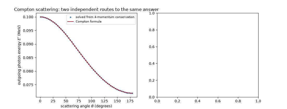
incident photon energy: 0.1 MeV
max |numeric - formula| across all angles: 8.41e-14 MeV
at theta=180 deg (backscatter): E' numeric = 0.071871 MeV, formula = 0.071871 MeV

<matplotlib.legend.Legend object at 0x16b70fa10>

The wavelength shift itself

lambda_shift = (1.0 / E_numeric) - (1.0 / E_incident)  # natural units: lambda = 1/E
lambda_shift_formula = (1.0 / m_e) * (1.0 - np.cos(theta_values))
ax2.plot(np.degrees(theta_values), lambda_shift, "o", ms=3, color="steelblue")
ax2.plot(np.degrees(theta_values), lambda_shift_formula, "-", color="firebrick")
ax2.set_xlabel(r"scattering angle $\theta$ (degrees)")
ax2.set_ylabel(r"$\lambda' - \lambda$ (MeV$^{-1}$, natural units)")
ax2.set_title(r"Wavelength shift depends only on $\theta$, not on target material")
fig.tight_layout()

plt.show()