Energy-conserving gyration with the Boris pusher

Jay Boris, developing early particle-in-cell plasma codes, needed a numerical integrator for the Lorentz force \(m\dot{\mathbf{v}}=q(\mathbf{E}+\mathbf{v}\times\mathbf{B})\) that would not spuriously heat or cool a particle over millions of simulated gyro-orbits. His 1970 scheme splits each leapfrog step into an electric half-kick, an exact rotation about \(\mathbf{B}\) computed without any trigonometry (the “Boris rotation” trick), and a second electric half-kick; the rotation step conserves speed to machine precision in a pure magnetic field, regardless of step size.

boris_push() and boris_integrate() implement the scheme with Numba-compiled kernels; physicskit.plasma.kinetic reuses the same leapfrog philosophy for its particle-in-cell push step.

import matplotlib.pyplot as plt
import numpy as np

import physicskit as pk

A proton gyrating in a 1 T field

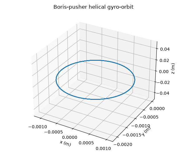
Resolve the gyro-period with 200 steps per orbit and integrate for 10 full orbits.

omega_c = pk.plasma.cyclotron_frequency(pk.plasma.QE, pk.plasma.MP, 1.0)
dt = (2 * np.pi / omega_c) / 200
pos_hist, vel_hist = pk.plasma.boris_integrate(
    np.zeros(3),
    np.array([1e5, 0.0, 0.0]),
    pk.plasma.QE,
    pk.plasma.MP,
    np.zeros(3),
    np.array([0.0, 0.0, 1.0]),
    dt=dt,
    steps=2000,
)

Speed is conserved to machine precision over every gyration – the Boris rotation trick, not accuracy of the time step, is why.

speeds = np.linalg.norm(vel_hist, axis=1)
print("max speed drift:", np.max(np.abs(speeds - 1e5)))

fig = plt.figure(figsize=(6, 5))
ax = fig.add_subplot(projection="3d")
pk.plasma.plot_particle_orbit_3d(pos_hist, ax=ax)
ax.set_title("Boris-pusher helical gyro-orbit")
fig.tight_layout()

plt.show()

max speed drift: 1.3096723705530167e-10

Making the conservation claim visible, not just printed

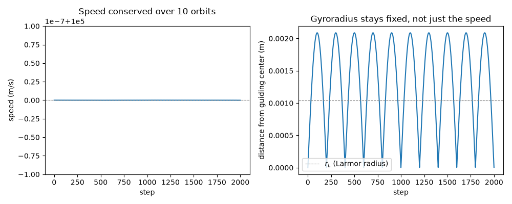
The single number above is easy to trust and hard to picture. Reusing the same speeds array over all 2000 steps – no extra integration – shows the speed staying flat to within machine precision for every one of the ten orbits, and comparing the particle’s radial distance from the guiding center (which sits at the origin here, since there is no E field or drift) against the closed-form gyroradius from larmor_radius() confirms the orbit traces the exact same circle every gyration instead of slowly spiraling in or out.

r_L = pk.plasma.larmor_radius(1e5, pk.plasma.QE, pk.plasma.MP, 1.0)
r_hist = np.linalg.norm(pos_hist[:, :2], axis=1)

fig, axes = plt.subplots(1, 2, figsize=(10, 4))
axes[0].plot(speeds)
axes[0].axhline(1e5, color="gray", linestyle="--", linewidth=0.8)
axes[0].set_xlabel("step")
axes[0].set_ylabel("speed (m/s)")
axes[0].set_title("Speed conserved over 10 orbits")

axes[1].plot(r_hist)
axes[1].axhline(r_L, color="gray", linestyle="--", linewidth=0.8, label=r"$r_L$ (Larmor radius)")
axes[1].set_xlabel("step")
axes[1].set_ylabel("distance from guiding center (m)")
axes[1].set_title("Gyroradius stays fixed, not just the speed")
axes[1].legend()
fig.tight_layout()

plt.show()