Recovering the ExB drift as a time-average of the full orbit

Modern magnetic-confinement fusion research is dominated by gyrokinetic theory: rather than track a particle’s full gyration (as the Boris pusher does, Energy-conserving gyration with the Boris pusher) or reduce all the way to a fluid (as MHD does), gyrokinetics analytically averages the Vlasov equation over the fast gyro-angle while retaining the finite-Larmor-radius physics needed for turbulence. This closes the gap between the guiding-center drift theory of the 1950s (Guiding-center drifts and magnetic mirror confinement) and full kinetic simulation, and is the theoretical foundation of every modern turbulent-transport code (GENE, GYRO, GS2) used to predict a fusion reactor’s confinement performance.

The guiding-center machinery in physicskit.plasma.single_particle – drifts, the adiabatic invariant, mirror bounce motion – is precisely the single-particle foundation gyrokinetic theory builds on. This script makes that connection concrete: the closed-form guiding-center prediction

\[\mathbf{v}_E = \frac{\mathbf{E}\times\mathbf{B}}{B^2}\]

from exb_drift() – independent of the particle’s charge, mass, and gyro-phase – is recovered by time-averaging a full orbit that integrates the exact Lorentz force \(m\dot{\mathbf{v}}=q(\mathbf{E}+\mathbf{v}\times\mathbf{B})\) with the Boris pusher: a uniform crossed \(\mathbf{E}\) and \(\mathbf{B}\) field are applied to a charged particle started from rest, and its gyrating-and-drifting trajectory is averaged over many gyro-periods – exactly the gyro-average gyrokinetics performs analytically.

import matplotlib.pyplot as plt
import numpy as np

import physicskit as pk

The closed-form guiding-center prediction: pure E x B drift

Independent of the particle’s gyro-phase, mass, or charge.

E = np.array([0.0, 1e3, 0.0])
B = np.array([0.0, 0.0, 1.0])
v_exb = pk.plasma.exb_drift(E, B)

The full Boris-pusher orbit gyrates and drifts; averaging its trajectory over many gyro-periods recovers the same drift velocity that gyrokinetic theory retains after averaging away the gyration.

omega_c = pk.plasma.cyclotron_frequency(pk.plasma.QE, pk.plasma.MP, 1.0)
dt = (2 * np.pi / omega_c) / 200
pos_hist, vel_hist = pk.plasma.boris_integrate(np.zeros(3), np.zeros(3), pk.plasma.QE, pk.plasma.MP, E, B, dt, steps=4000)
v_avg = (pos_hist[-1] - pos_hist[0]) / (4000 * dt)
print("guiding-center v_ExB:", v_exb)
print("full-orbit time-averaged velocity:", v_avg)

fig, ax = plt.subplots(figsize=(6, 5))
pk.plasma.plot_drift_trajectory(pos_hist, ax=ax)
ax.set_title("Full gyro-orbit drifting at the guiding-center ExB speed")
fig.tight_layout()

plt.show()

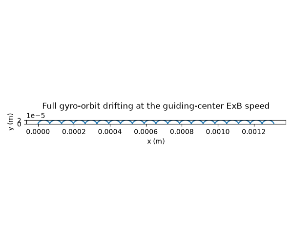
guiding-center v_ExB: [1000.    0.    0.]
full-orbit time-averaged velocity: [ 1.00008224e+03 -8.66816231e-04  0.00000000e+00]

The gyro-average made visible: a velocity-space hodograph

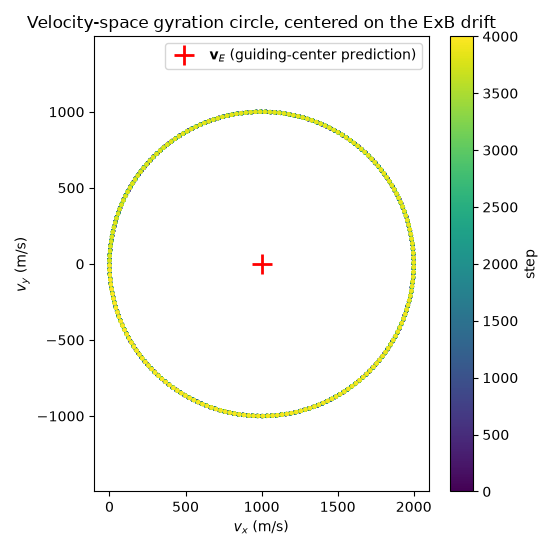
Time-averaging the position history above recovers the drift speed, but the gyroaveraging gyrokinetics performs is really an average over velocity space: the full velocity subtracts into a fast gyration circling a fixed center plus the slow drift. Reusing the same vel_hist already returned by boris_integrate() – no new integration needed – and plotting \(v_x\) against \(v_y\) traces exactly that circle, centered on the closed-form \(\mathbf{v}_E\) from exb_drift() rather than on the origin: the gyration is what gyrokinetics averages away, and the offset center is what survives the average.

fig, ax = plt.subplots(figsize=(5.5, 5.5))
sc = ax.scatter(vel_hist[:, 0], vel_hist[:, 1], c=np.arange(len(vel_hist)), cmap="viridis", s=4)
fig.colorbar(sc, ax=ax, label="step")
ax.plot(v_exb[0], v_exb[1], "r+", markersize=14, markeredgewidth=2, label=r"$\mathbf{v}_E$ (guiding-center prediction)")
ax.set_xlabel(r"$v_x$ (m/s)")
ax.set_ylabel(r"$v_y$ (m/s)")
ax.set_title("Velocity-space gyration circle, centered on the ExB drift")
ax.set_aspect("equal", adjustable="datalim")
ax.legend()
fig.tight_layout()

plt.show()