The Kerr shadow: a rotating black hole’s asymmetric silhouette

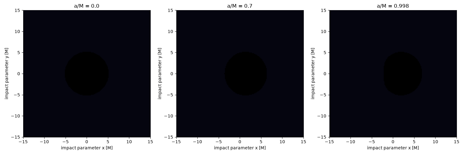
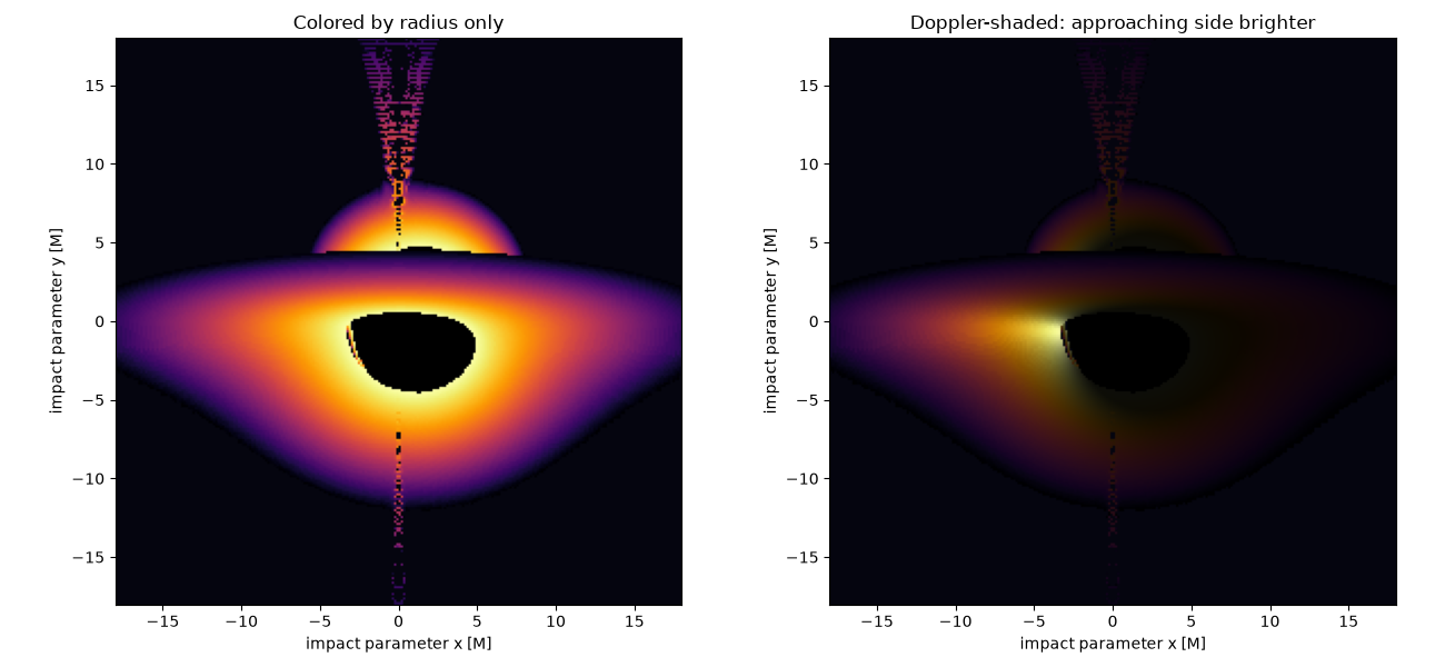
A rotating black hole’s shadow is not a perfect circle like Schwarzschild’s: frame dragging shifts and flattens it along the direction of rotation, and the accretion disk’s approaching side is Doppler-boosted bright while the receding side dims – exactly the asymmetric brightness pattern seen in the 2019 Event Horizon Telescope image of M87*. This example ray-traces the full (non-equatorial) Kerr null geodesic equations – using Carter’s separated equations of motion in Mino time – to render the shadow of a black hole of mass \(M\) and spin parameter \(a\) at increasing spin, and shades a thin, circularly orbiting equatorial accretion disk by its combined gravitational and Doppler redshift

\[g = \frac{E_{\text{obs}}}{E_{\text{emit}}} = \frac{1}{u^t(r)\left[1 - b\,\Omega(r)\right]}\]

where \(b = L_{\text{ph}}/E_{\text{ph}}\) is the received photon’s impact parameter, \(\Omega(r)\) is the disk’s Keplerian angular velocity, and \(u^t(r)\) is the emitting gas’s time-dilation factor; \(g>1\) (blueshifted) marks the approaching side and \(g<1\) (redshifted) the receding side. Rendered brightness is further boosted by \(g^3\), the relativistic Doppler-beaming factor for a locally isotropic emitter.

import matplotlib.pyplot as plt

from physicskit.relativity.visualizers.shadow_render import plot_black_hole_shadow, render_black_hole_image

The shadow shrinks and shifts as spin increases

fig, axes = plt.subplots(1, 3, figsize=(15, 5))
for ax, a in zip(axes, [0.0, 0.7, 0.998]):
    result = render_black_hole_image(M=1.0, a=a, ny=180, nx=180, inclination=1.3, r_disk_inner=1.0, r_disk_outer=0.0)
    plot_black_hole_shadow(result, ax=ax)
    ax.set_title(f"a/M = {a}")
plt.tight_layout()

A redshift-shaded accretion disk (near-extremal spin, oblique view)

result = render_black_hole_image(M=1.0, a=0.9, ny=250, nx=250, inclination=1.35, screen_half_width=18.0)
fig, axes = plt.subplots(1, 2, figsize=(13, 6))
plot_black_hole_shadow(result, ax=axes[0], redshift=False)
axes[0].set_title("Colored by radius only")
plot_black_hole_shadow(result, ax=axes[1], redshift=True)
axes[1].set_title("Doppler-shaded: approaching side brighter")
plt.tight_layout()
plt.show()