Herman-Kluk frozen-Gaussian wavepacket propagation

Michael Herman and Edward Kluk’s 1984 method propagates a quantum wavepacket by summing many classical trajectories rather than following just one: launch one fixed-width (“frozen”) Gaussian wavepacket from every point of a phase-space grid under the initial state, propagate each one along its own classical trajectory, and sum the results with a monodromy-built prefactor and classical action phase,

\[\psi(x,t) \approx \int\!\frac{dq_0\,dp_0}{2\pi\hbar}\, C_t(q_0,p_0)\,e^{iS(t)/\hbar}\, \langle g_{q_0,p_0}|\psi_0\rangle\, g_{q_t,p_t}(x),\]

(herman_kluk_propagate_wavepacket(), built on frozen_gaussian_1d() and the monodromy-built prefactor \(C_t\), herman_kluk_prefactor()). Unlike the single-trajectory Van Vleck-Morette propagator (The Van Vleck-Morette semiclassical propagator), this multi-trajectory (“initial value representation”) sum needs no troublesome root-finding to connect fixed endpoints, and – for a potential at most quadratic in position, as here – is exact.

Propagates an initial frozen-Gaussian (coherent) wavepacket centered at \((q_c,p_c)=(2.0,0.0)\) for a unit-mass, unit-frequency harmonic oscillator, \(V(q)=\tfrac12m\omega^2q^2\) with \(m=\omega=1\), and compares the propagated wavepacket at \(t=T/2\) (half an oscillator period) to the exact analytic coherent-state evolution.

import matplotlib.pyplot as plt
import numpy as np
from numba import njit

from physicskit.quantum.chapters.harmonic_spin import HarmonicOscillator
from physicskit.semiclassical.core.propagators import herman_kluk_propagate_wavepacket

m, omega = 1.0, 1.0
params = np.array([m * omega**2])


@njit(cache=True)
def dVdx(q, params):
    return params[0] * q


@njit(cache=True)
def d2Vdx2(q, params):
    return params[0]


@njit(cache=True)
def V(q, params):
    return 0.5 * params[0] * q**2


T_period = 2 * np.pi / omega

ho = HarmonicOscillator()
gamma = 1.0 / (2 * ho.x0**2)

qc0, pc0 = 2.0, 0.0
alpha = qc0 / (ho.x0 * np.sqrt(2)) + 1j * pc0 / np.sqrt(2 * ho.hbar * ho.m * ho.omega)

t_hk = 0.5 * T_period
steps_hk = 2000
x_eval = np.linspace(-6, 6, 400)

psi_hk = herman_kluk_propagate_wavepacket(
    qc0, pc0, gamma, dVdx, d2Vdx2, V, ho.m, dt=t_hk / steps_hk, steps=steps_hk, x_eval=x_eval, hbar=ho.hbar, n_grid=51, n_sigma=6.0, params=params
)
psi_exact = ho.coherent_wavefunction(alpha, x_eval, t=t_hk)

The Herman-Kluk multi-trajectory propagator vs. the exact coherent-state evolution ————————————————————————

fig, ax = plt.subplots(figsize=(6.5, 4.5))
ax.plot(x_eval, np.abs(psi_exact) ** 2, label="exact coherent state |psi(t)|^2")
ax.plot(x_eval, np.abs(psi_hk) ** 2, "--", label="Herman-Kluk |psi(t)|^2")
ax.set_xlabel("x")
ax.set_title("Herman-Kluk vs. exact coherent-state evolution at t=T/2")
ax.legend(fontsize=8)
fig.tight_layout()

overlap = np.abs(np.trapezoid(np.conj(psi_exact) * psi_hk, x_eval)) ** 2
print(f"Herman-Kluk fidelity to the exact coherent state at t=T/2: {overlap:.4f}")

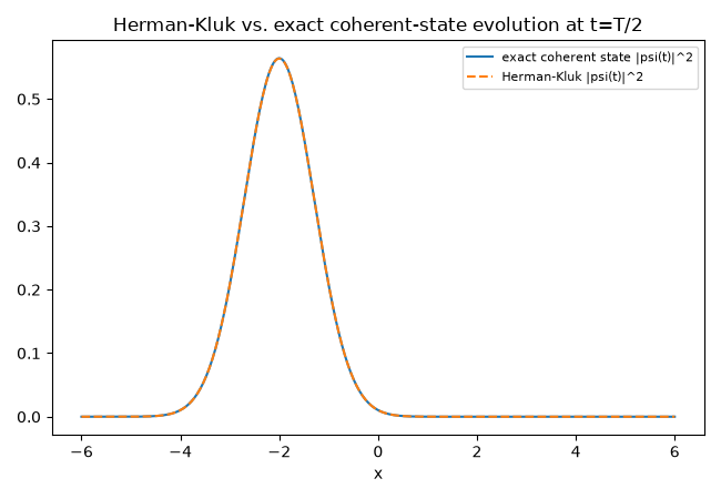
Herman-Kluk fidelity to the exact coherent state at t=T/2: 0.9999