The Fokker-Planck equation: from noisy trajectories to a deterministic density

Adriaan Fokker (1914) and Max Planck (1917) replaced the random path of a Brownian particle with an equation for its probability density. For \(dX = A(X)\,dt + \sqrt{2D}\,dW\),

\[\frac{\partial p}{\partial t} = -\frac{\partial}{\partial x}\big[A(x)\,p\big] + D\,\frac{\partial^2 p}{\partial x^2}.\]

The randomness has gone: \(p\) evolves deterministically. For an overdamped particle in a potential, \(A = -U'/\gamma\) and \(D = k_BT/\gamma\), the density relaxes to the Boltzmann distribution \(e^{-U/k_BT}/Z\).

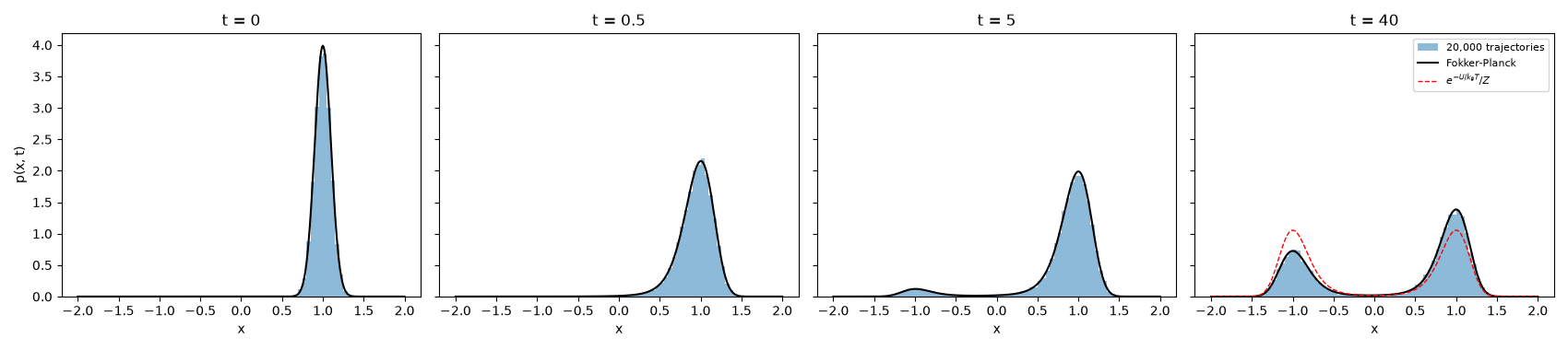
This example puts particles in the double well \(U = (x^2 - 1)^2\), all starting in the right-hand well. It follows them two ways: 20,000 Langevin trajectories, integrated with euler_maruyama_integrate(), and one Fokker-Planck solve with fokker_planck_1d(). The histogram and the density agree at every time as the population leaks over the barrier to fill both wells.

import matplotlib.pyplot as plt
import numpy as np
from numba import njit

from physicskit.integrators import euler_maruyama_integrate, wiener_increments
from physicskit.statphys import fokker_planck_1d, fokker_planck_stationary

gamma, kT = 1.0, 0.25


@njit
def double_well_drift(x, t, p):
    return -4.0 * x * (x * x - 1.0) / p[0]


@njit
def thermal_noise(x, t, p):
    return np.sqrt(2.0 * p[1] / p[0]) * np.ones_like(x)

Trajectories and density side by side

n, dt = 20000, 0.002
frames = [0.0, 0.5, 5.0, 40.0]
x = np.linspace(-2.0, 2.0, 401)
x0 = 1.0 + 0.1 * np.random.default_rng(1914).standard_normal(n)
p0 = np.exp(-((x - 1.0) ** 2) / (2 * 0.1**2))
drift = lambda y: -4.0 * y * (y**2 - 1.0) / gamma

samples = [x0]
state = x0.copy()
rng = np.random.default_rng(1917)
chunk = 250  # draw the noise a chunk at a time rather than all at once
for t_prev, t_next in zip(frames[:-1], frames[1:]):
    for c in range(round((t_next - t_prev) / dt) // chunk):
        dW = wiener_increments(chunk, n, dt, rng=rng)
        _, traj = euler_maruyama_integrate(double_well_drift, thermal_noise, state, t_prev + c * chunk * dt, dt, dW, np.array([gamma, kT]), chunk)
        state = traj[-1]
    samples.append(state)

densities = [p0 / (p0.sum() * (x[1] - x[0]))]
for t_prev, t_next in zip(frames[:-1], frames[1:]):
    _, p = fokker_planck_1d(densities[-1], x, drift, kT / gamma, t_max=t_next - t_prev, dt=0.01, n_frames=1)
    densities.append(p[-1])

boltzmann = fokker_planck_stationary(x, drift, kT / gamma)
for t_f, xs, p in zip(frames, samples, densities):
    left_traj = np.mean(xs < 0)
    left_fp = np.sum(p[x < 0]) * (x[1] - x[0])
    print(f"t = {t_f:5.1f}: fraction in the left well, trajectories {left_traj:.3f}, Fokker-Planck {left_fp:.3f}")

t =   0.0: fraction in the left well, trajectories 0.000, Fokker-Planck 0.000
t =   0.5: fraction in the left well, trajectories 0.004, Fokker-Planck 0.003
t =   5.0: fraction in the left well, trajectories 0.068, Fokker-Planck 0.065
t =  40.0: fraction in the left well, trajectories 0.350, Fokker-Planck 0.346

The escape rate

The left-well population approaches 1/2 as \(\tfrac12(1 - e^{-2kt})\). At low temperature, Kramers (1940) gives the hopping rate \(k \approx \frac{\sqrt{U''(x_{\min})|U''(x_{\max})|}}{2\pi\gamma} e^{-\Delta U/k_BT}\), with barrier \(\Delta U = 1\) here.

t_long, p_long = fokker_planck_1d(densities[0], x, drift, kT / gamma, t_max=40.0, dt=0.01, n_frames=200)
left = np.sum(p_long[:, x < 0], axis=1) * (x[1] - x[0])
fit = (t_long > 5) & (t_long < 30)
rate = -0.5 * np.polyfit(t_long[fit], np.log(1 - 2 * left[fit]), 1)[0]
kramers = np.sqrt(8.0 * 4.0) / (2 * np.pi * gamma) * np.exp(-1.0 / kT)
print(f"hopping rate: Fokker-Planck {rate:.4f}, Kramers estimate {kramers:.4f}")

fig, axes = plt.subplots(1, 4, figsize=(17, 3.8), sharey=True)
for ax, t_f, xs, p in zip(axes, frames, samples, densities):
    ax.hist(xs, bins=np.linspace(-2, 2, 81), density=True, alpha=0.5, label="20,000 trajectories")
    ax.plot(x, p, "k", lw=1.5, label="Fokker-Planck")
    if t_f == frames[-1]:
        ax.plot(x, boltzmann, "r--", lw=1, label=r"$e^{-U/k_BT}/Z$")
    ax.set_title(f"t = {t_f:g}")
    ax.set_xlabel("x")
axes[0].set_ylabel("p(x, t)")
axes[-1].legend(fontsize=8)
fig.tight_layout()

fig2, ax2 = plt.subplots(figsize=(6, 4))
ax2.plot(t_long, left, label="Fokker-Planck")
ax2.plot(t_long, 0.5 * (1 - np.exp(-2 * rate * t_long)), "k--", lw=1, label=rf"$\frac{{1}}{{2}}(1 - e^{{-2kt}})$, $k$ = {rate:.3f}")
ax2.set_xlabel("t")
ax2.set_ylabel("population of the left well")
ax2.set_title("barrier crossing")
ax2.legend()
fig2.tight_layout()
plt.show()

• 
• 

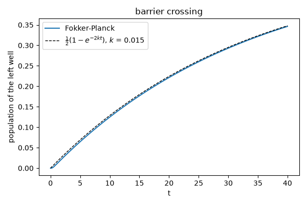
hopping rate: Fokker-Planck 0.0149, Kramers estimate 0.0165

Check

Trajectories and the Fokker-Planck solution agree; the well populations relax as 1/2 (1 - e^(-2kt)) toward the symmetric Boltzmann state; the hopping rate matches Kramers’ estimate sqrt(U’’(min) |U''(max)|) / (2 pi gamma) e^(-Delta U / kT) to ~15%.

for xs, p in zip(samples, densities):
    assert abs(np.mean(xs < 0) - np.sum(p[x < 0]) * (x[1] - x[0])) < 0.01
assert np.max(np.abs(left[fit] - 0.5 * (1 - np.exp(-2 * rate * t_long[fit])))) < 0.01
assert abs(np.sum(boltzmann[x < 0]) / np.sum(boltzmann) - 0.5) < 0.01
assert abs(rate / kramers - 1) < 0.15