Itô’s stochastic calculus: the Euler-Maruyama and Milstein schemes

Kiyosi Itô (1944) gave meaning to integrals against Brownian motion, and with them to stochastic differential equations \(dX = a(X)\,dt + b(X)\,dW\). The key rule is that \(dW^2 = dt\), not zero. As a result, \(\ln X\) for geometric Brownian motion \(dX = \mu X\,dt + \sigma X\,dW\) drifts at \(\mu - \sigma^2/2\) rather than \(\mu\), and the exact solution is

\[X_t = X_0\exp\!\big[(\mu - \tfrac12\sigma^2)t + \sigma W_t\big].\]

Maruyama (1955) proved that the obvious discretization, \(X_{n+1} = X_n + a\,\Delta t + b\,\Delta W\), converges to Itô’s solution, but only as \(\Delta t^{1/2}\) path by path. Milstein (1974) added the term \(\tfrac12 b b'(\Delta W^2 - \Delta t)\) from Itô’s formula and raised the order to 1.

This example drives euler_maruyama_integrate() and milstein_integrate() with the same Brownian paths at coarser and coarser steps. It measures both orders against the exact solution, and shows the \(-\sigma^2/2\) Itô drift.

import matplotlib.pyplot as plt
import numpy as np
from numba import njit

from physicskit.integrators import euler_maruyama_integrate, milstein_integrate, wiener_increments

mu, sigma, T = 0.3, 0.9, 1.0
params = np.array([mu, sigma])


@njit
def gbm_drift(x, t, p):
    return p[0] * x


@njit
def gbm_diffusion(x, t, p):
    return p[1] * x


@njit
def gbm_diffusion_derivative(x, t, p):
    return p[1] * np.ones_like(x)

One path at three resolutions

Coarser increments are sums of the fine ones, so all three runs feel exactly the same noise.

n_fine, n_paths = 2**12, 2000
dW = wiener_increments(n_fine, n_paths, T / n_fine, rng=1955)
W = np.vstack([np.zeros(n_paths), np.cumsum(dW, axis=0)])
t_fine = np.linspace(0, T, n_fine + 1)
exact_path = np.exp((mu - 0.5 * sigma**2) * t_fine + sigma * W[:, 0])
x0 = np.ones(n_paths)

Strong convergence orders

steps = 2 ** np.arange(3, 11)
err_em, err_mil = [], []
exact_T = np.exp((mu - 0.5 * sigma**2) * T + sigma * W[-1])
coarse = {}
for n in steps:
    dW_n = dW.reshape(n, n_fine // n, n_paths).sum(axis=1)
    t_n, em = euler_maruyama_integrate(gbm_drift, gbm_diffusion, x0, 0.0, T / n, dW_n, params)
    _, mil = milstein_integrate(gbm_drift, gbm_diffusion, gbm_diffusion_derivative, x0, 0.0, T / n, dW_n, params)
    err_em.append(np.mean(np.abs(em[-1] - exact_T)))
    err_mil.append(np.mean(np.abs(mil[-1] - exact_T)))
    if n in (8, 64):
        coarse[n] = (t_n, em[:, 0], mil[:, 0])
dts = T / steps
order_em = np.polyfit(np.log(dts), np.log(err_em), 1)[0]
order_mil = np.polyfit(np.log(dts), np.log(err_mil), 1)[0]
print(f"strong order: Euler-Maruyama {order_em:.2f} (theory 0.5), Milstein {order_mil:.2f} (theory 1.0)")

strong order: Euler-Maruyama 0.50 (theory 0.5), Milstein 0.95 (theory 1.0)

The Itô correction

The mean of \(\ln X_T\) is \((\mu - \sigma^2/2)T\), not \(\mu T\), while the mean of \(X_T\) itself grows as \(e^{\mu T}\).

se_log = np.std(np.log(exact_T)) / np.sqrt(n_paths)
se_x = np.std(exact_T) / np.sqrt(n_paths)
print(f"<ln X_T> = {np.mean(np.log(exact_T)):.3f} +/- {se_log:.3f}; (mu - sigma^2/2) T = {(mu - 0.5 * sigma**2) * T:.3f}; mu T = {mu * T:.3f}")
print(f"<X_T> = {np.mean(exact_T):.3f} +/- {se_x:.3f}; exp(mu T) = {np.exp(mu * T):.3f}")

fig, axes = plt.subplots(1, 3, figsize=(15, 4.3))
axes[0].plot(t_fine, exact_path, "k", lw=1, label="exact")
for n, style in ((8, "o-"), (64, "-")):
    t_n, em, mil = coarse[n]
    axes[0].plot(t_n, em, style, ms=3, lw=0.8, color="tab:orange", label=f"Euler-Maruyama, {n} steps")
    axes[0].plot(t_n, mil, style, ms=3, lw=0.8, color="tab:blue", label=f"Milstein, {n} steps")
axes[0].set_xlabel("t")
axes[0].set_ylabel("X")
axes[0].set_title("one geometric Brownian path")
axes[0].legend(fontsize=7)

axes[1].loglog(dts, err_em, "o-", color="tab:orange", label=f"Euler-Maruyama, slope {order_em:.2f}")
axes[1].loglog(dts, err_mil, "s-", color="tab:blue", label=f"Milstein, slope {order_mil:.2f}")
axes[1].loglog(dts, err_em[0] * (dts / dts[0]) ** 0.5, "k:", lw=1)
axes[1].loglog(dts, err_mil[0] * (dts / dts[0]), "k--", lw=1)
axes[1].set_xlabel(r"$\Delta t$")
axes[1].set_ylabel(r"$\langle |X_T - X_T^{\rm exact}|\rangle$")
axes[1].set_title("strong error")
axes[1].legend(fontsize=8)

lx = np.log(exact_T)
axes[2].hist(lx, bins=60, density=True, alpha=0.6)
axes[2].axvline((mu - 0.5 * sigma**2) * T, color="k", ls="--", label=r"$(\mu - \sigma^2/2)T$ (Itô)")
axes[2].axvline(mu * T, color="firebrick", ls=":", label=r"$\mu T$ (naive)")
axes[2].set_xlabel(r"$\ln X_T$")
axes[2].set_title("the Itô drift correction")
axes[2].legend(fontsize=8)
fig.tight_layout()
plt.show()

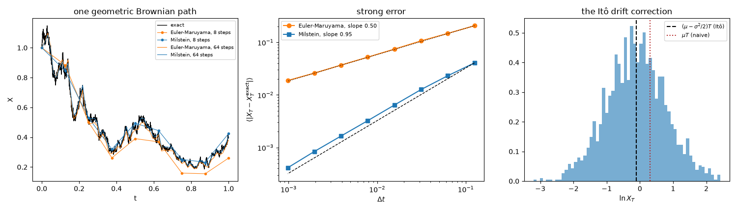
<ln X_T> = -0.118 +/- 0.020; (mu - sigma^2/2) T = -0.105; mu T = 0.300
<X_T> = 1.314 +/- 0.030; exp(mu T) = 1.350

Check

Strong orders 1/2 (Euler-Maruyama) and 1 (Milstein); the Ito drift correction: <ln X_T> = (mu - sigma^2/2) T, while <X_T> = e^(mu T).

assert abs(order_em - 0.5) < 0.1 and abs(order_mil - 1.0) < 0.1
assert abs(np.mean(np.log(exact_T)) - (mu - 0.5 * sigma**2) * T) < 3 * se_log
assert abs(np.mean(exact_T) - np.exp(mu * T)) < 3 * se_x