Breakthroughs in Exotic Options#

financialkit.exotic_options hub · History · Examples · API reference

“In physics you’re playing against God; in finance you’re playing against God’s creatures.” – attributed to Emanuel Derman

The Black-Scholes argument prices any payoff that a dynamic hedge can replicate, and within months of its publication Merton had used it on a contract nobody traded yet: a call that dies at a barrier. Through the 1980s the over-the-counter market caught up with the theory. Banks sold options on averages to commodity users, options on the better of two assets to fund managers and options paid in another currency to investors who wanted foreign stocks without foreign exchange risk. Most of the closed forms were collected, and many were found, by Mark Rubinstein and Eric Reiner in a run of short articles in Risk in 1991. The later breakthroughs are numerical: correcting continuous formulas for discrete monitoring, replicating volatility itself, and pricing early exercise by simulation. This chronology traces the ideas behind financialkit.exotic_options.

1973 – Merton’s Down-and-Out Call #

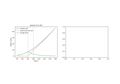
In “Theory of Rational Option Pricing” Robert Merton put the Black-Scholes model on an arbitrage footing and, almost in passing, priced the first exotic option: a call that is cancelled if the stock falls to a level \(H\) below the strike. The barrier is an absorbing boundary for the log-price, and the method of images from the heat equation removes the paths that touch it: subtract the value of a call started from the reflected spot \(H^2/S\), scaled to make the price vanish on the barrier.

\[C_{do}(S) = c(S, K) - \left(\frac{H}{S}\right)^{2b/\sigma^2 - 1} c\!\left(\frac{H^2}{S}, K\right), \qquad b = r - q\]

Implementation: financialkit.exotic_options.systems.barriers.merton_down_and_out_call() evaluates the image formula with financialkit.options.black_scholes_price(). The example compares it with the vanilla call for several barriers and checks it against bridge-corrected Monte Carlo (barrier_option_mc()).

References: R. C. Merton, “Theory of Rational Option Pricing,” Bell Journal of Economics and Management Science 4 (1973) 141-183, Section 8.

Merton’s down-and-out call

Merton's down-and-out call

1978 – Margrabe’s Exchange Option #

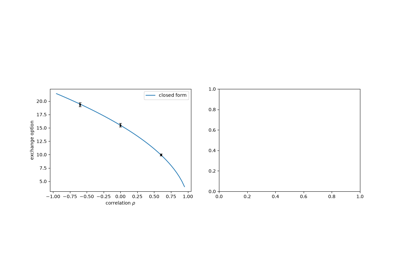
William Margrabe priced the right to exchange one risky asset for another at maturity. Measured in units of the asset given up, the payoff is a call on the ratio of the two prices struck at one; the ratio is lognormal with volatility \(\sigma^2 = \sigma_1^2 + \sigma_2^2 - 2\rho\sigma_1\sigma_2\), and the interest rate disappears from the answer. The proof by change of numeraire, one of the first, became a standard tool, and the formula prices spread options, outperformance options and the switching options embedded in many contracts.

\[V = S_1 e^{-q_1 T} N(d_1) - S_2 e^{-q_2 T} N(d_2), \qquad d_{1,2} = \frac{\ln(S_1 e^{-q_1 T}/S_2 e^{-q_2 T}) \pm \tfrac12\sigma^2 T}{\sigma\sqrt T}\]

Implementation: financialkit.exotic_options.systems.multi_asset.margrabe_price() calls financialkit.options.black_scholes_price() with the second asset as strike and a zero rate. The example plots the price against the correlation, with correlated Monte Carlo from financialkit.integrators.correlated_increments().

References: W. Margrabe, “The Value of an Option to Exchange One Asset for Another,” Journal of Finance 33 (1978) 177-186.

Margrabe exchange options

1979 – Goldman-Sosin-Gatto Floating Lookbacks #

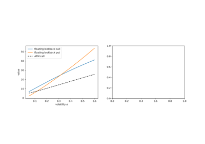
“Path Dependent Options: Buy at the Low, Sell at the High” by Barry Goldman, Howard Sosin and Mary Ann Gatto priced the option that lets its holder buy at the lowest price of the option’s life, \(S_T - \min_t S_t\), or sell at the highest. It is never out of the money. The joint law of a Brownian motion with drift and its running minimum, from the reflection principle, gives the closed form.

\[c = S e^{(b-r)T} N(a_1) - S_{\min} e^{-rT} N(a_2) + S e^{-rT}\frac{\sigma^2}{2b}\left[\left(\frac{S}{S_{\min}}\right)^{-2b/\sigma^2} N\!\left(-a_1 + \frac{2b\sqrt T}{\sigma}\right) - e^{bT} N(-a_1)\right]\]

Implementation: financialkit.exotic_options.systems.lookbacks.floating_lookback_price() prices new and seasoned floating lookbacks, taking the zero-carry limit where the formula is singular, and lookback_option_mc() simulates them with each step’s extremum drawn exactly from the Brownian bridge (bridge_extremum()). The example contrasts this with the biased minimum over a grid.

References: M. B. Goldman, H. B. Sosin and M. A. Gatto, “Path Dependent Options: ‘Buy at the Low, Sell at the High’,” Journal of Finance 34 (1979) 1111-1127.

Goldman-Sosin-Gatto floating lookbacks

1979 – Geske’s Compound Options #

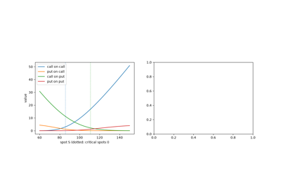
Robert Geske priced an option on an option. His motivation was corporate finance: if a levered firm’s equity is a call on its assets, then a stock option is a call on a call, and its Black-Scholes volatility should change with the stock price. The compound call is exercised at \(T_1\) when the underlying option is worth more than its strike, which happens above a critical spot \(I\), and the joint law of the price at the two expiries brings in the bivariate normal distribution with correlation \(\sqrt{T_1/T_2}\).

\[C = S e^{-qT_2} M(z_1, y_1; \rho) - K_2 e^{-rT_2} M(z_2, y_2; \rho) - K_1 e^{-rT_1} N(y_2), \qquad \rho = \sqrt{T_1/T_2}\]

Implementation: financialkit.exotic_options.systems.compound.compound_option_price() prices all four combinations of calls and puts, finding the critical spot with scipy.optimize.brentq() (critical_price()) and the bivariate normal exactly from Owen’s T function (bivariate_normal_cdf()). The example plots the four options and checks compound put-call parity.

References: R. Geske, “The Valuation of Compound Options,” Journal of Financial Economics 7 (1979) 63-81.

Geske compound options

1982 – Stulz: Options on the Maximum and the Minimum #

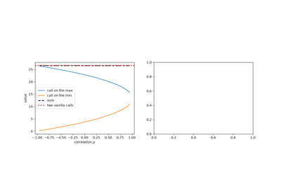
Rene Stulz priced European calls and puts on the larger or the smaller of two lognormal assets, the first “rainbow” options. The answer is a combination of bivariate normal probabilities. Because the maximum and the minimum add up to the two assets, a call on the maximum and a call on the minimum together are worth the two vanilla calls, and the correlation only moves value between them: the less correlated the assets, the more the maximum is worth.

\[c_{\min} = S_1 e^{-q_1 T} M(y_1, -d; -\rho_1) + S_2 e^{-q_2 T} M(y_2, d - \sigma\sqrt T; -\rho_2) - K e^{-rT} M(y_1 - \sigma_1\sqrt T, y_2 - \sigma_2\sqrt T; \rho)\]

Implementation: financialkit.exotic_options.systems.multi_asset.stulz_price() prices calls and puts on the maximum and the minimum, the puts by parity with the zero-strike call, a Margrabe option. The example shows the calls against the correlation and the puts against the strike.

References: R. M. Stulz, “Options on the Minimum or the Maximum of Two Risky Assets: Analysis and Applications,” Journal of Financial Economics 10 (1982) 161-185.

Stulz options on the maximum and minimum

1990 – Kemna-Vorst Asian Options #

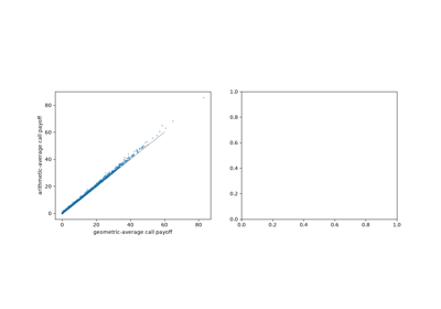
Average-rate options suit firms that buy or sell a commodity steadily and are harder to manipulate at expiry. Angelien Kemna and Ton Vorst noticed that the geometric average of lognormal prices is itself lognormal, with volatility \(\sigma/\sqrt3\) under continuous averaging, so its option has a Black-Scholes formula. The arithmetic average that contracts use has no closed form, but its option is so tightly correlated with the geometric one that the latter makes an almost perfect Monte Carlo control variate.

\[\ln G \sim N\!\left(\ln S + \left(b - \tfrac{\sigma^2}{2}\right)\tfrac{T}{2},\; \tfrac{\sigma^2 T}{3}\right), \qquad \hat\mu = \bar Y_{\text{arith}} - \beta(\bar Y_{\text{geo}} - V_{\text{geo}})\]

Implementation: financialkit.exotic_options.systems.asian.geometric_asian_price() prices continuous and discrete geometric averages, and arithmetic_asian_mc() simulates the arithmetic average with the geometric control through financialkit.monte_carlo.control_variate_estimate(). The example shows the two payoffs on common paths and the resulting variance reduction.

References: A. G. Z. Kemna and A. C. F. Vorst, “A Pricing Method for Options Based on Average Asset Values,” Journal of Banking and Finance 14 (1990) 113-129.

Kemna-Vorst Asian options

1990 – Rubinstein’s Forward-Start Options #

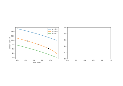
A forward-start option is struck at a fixed fraction \(\alpha\) of the price on a future date \(t\), the way executive options are granted at the money. Mark Rubinstein observed that on the start date it is worth the price times an option on a unit spot, so today it is worth \(S e^{-qt}\) times that option, whatever happens before \(t\). Its value is linear in the spot, it has no gamma until it starts, and a chain of them is a cliquet.

\[V = S e^{-qt}\,\mathrm{BS}(1, \alpha, T - t, r, q, \sigma)\]

Implementation: financialkit.exotic_options.systems.compound.forward_start_price(). The example plots the value against the start date with Monte Carlo checks and contrasts its linear profile with a vanilla call.

References: M. Rubinstein, “Exotic Options,” Finance working paper 220, University of California, Berkeley (1990); E. G. Haug, The Complete Guide to Option Pricing Formulas, 2nd ed. (McGraw-Hill, 2007), Section 4.3.

Rubinstein forward-start options

1991 – Reiner-Rubinstein Barrier Options #

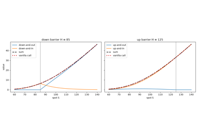
“Breaking Down the Barriers” by Eric Reiner and Mark Rubinstein gave closed forms for all eight single-barrier options – calls and puts, down and up, in and out – with a cash rebate paid at the hit for knock-outs or at expiry for knock-ins that never knock in. Each is a sum of six building blocks: the vanilla option, the vanilla struck at the barrier, their reflections and the two rebates. Without rebates a knock-in and the matching knock-out add up to the vanilla option, so barriers are a cheap way to buy only the scenarios one believes in.

\[C_{do} = A - C + F, \quad C_{di} = C + E \quad (K > H), \qquad V_{\text{in}} + V_{\text{out}} = V_{\text{vanilla}}\]

Implementation: financialkit.exotic_options.systems.barriers.barrier_price() implements all eight options with rebates, vectorised over spots and strikes. The example reproduces Haug’s Table 4-13 and plots in-out parity for down and up barriers.

References: E. Reiner and M. Rubinstein, “Breaking Down the Barriers,” Risk 4(8) (1991) 28-35; Haug (2007), Section 4.17.1.

Reiner-Rubinstein barrier options

1991 – Reiner-Rubinstein Binary Options #

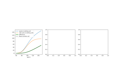
In “Unscrambling the Binary Code” Mark Rubinstein and Eric Reiner priced the all-or-nothing payoffs – cash-or-nothing, asset-or-nothing, gap and one-touch options – and showed that vanilla and barrier options decompose into them. The two terms of the Black-Scholes formula are exactly an asset-or-nothing call and \(K\) cash-or-nothing calls; a knock-out’s rebate is a one-touch.

\[c = \underbrace{S e^{-qT} N(d_1)}_{\text{asset-or-nothing}} - K \underbrace{e^{-rT} N(d_2)}_{\text{cash-or-nothing}}\]

Implementation: financialkit.exotic_options.systems.binaries.cash_or_nothing_price(), asset_or_nothing_price(), gap_option_price() and one_touch_price(). The example builds a call from two digitals, shows the digital’s delta spiking at the strike near expiry, and compares a one-touch with the digital that pays at expiry.

References: M. Rubinstein and E. Reiner, “Unscrambling the Binary Code,” Risk 4(9) (1991) 75-83; Haug (2007), Section 4.19.

Reiner-Rubinstein binary options

1991 – Rubinstein’s Chooser Options #

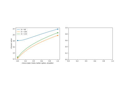
The holder of a simple chooser decides on a fixed date \(t\) whether the option is a call or a put, both with strike \(K\) and expiry \(T\). Put-call parity turns the choice into a call plus a put: at \(t\), \(\max(c, p) = c + (p - c)^+\), and \(p - c\) is the payoff of a forward. A chooser is worth the better option if the choice is made today and a straddle if it is made at expiry, which is the hedge a trader expecting a large move of unknown sign would buy.

\[V = c(S, K, T) + e^{-q(T-t)}\, p\big(S, K e^{-(r-q)(T-t)}, t\big)\]

Implementation: financialkit.exotic_options.systems.compound.chooser_price(). The example plots the value against the choice date between its two limits and checks the decision rule by Monte Carlo.

References: M. Rubinstein, “Options for the Undecided,” Risk 4(4) (1991) 43; Haug (2007), Section 4.4.1.

Rubinstein choosers

1991 – Conze-Viswanathan Fixed Lookbacks #

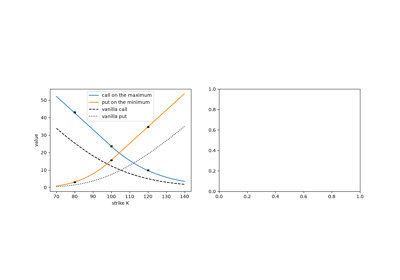
Antoine Conze and Viswanathan priced the fixed-strike lookback, a call on the maximum \((\max_t S_t - K)^+\) and a put on the minimum, together with seasoned options whose running extreme is already known. Once the maximum has passed the strike, the call has locked in \(\max - K\) and what remains is the value of further rises, so the same formula serves with \(S_{\max}\) in place of \(K\).

\[c = e^{-rT}(S_{\max} - K)^+ + S e^{(b-r)T}N(e_1) - M e^{-rT}N(e_2) + S e^{-rT}\frac{\sigma^2}{2b}\left[-\left(\frac{S}{M}\right)^{-2b/\sigma^2} N\!\left(e_1 - \frac{2b\sqrt T}{\sigma}\right) + e^{bT}N(e_1)\right], \quad M = \max(K, S_{\max})\]

Implementation: financialkit.exotic_options.systems.lookbacks.fixed_lookback_price(). The example prices new lookbacks across strikes against Monte Carlo and shows a seasoned call locking in its running maximum.

References: A. Conze and Viswanathan, “Path Dependent Options: The Case of Lookback Options,” Journal of Finance 46 (1991) 1893-1907; Haug (2007), Section 4.15.2.

Conze-Viswanathan fixed lookbacks

1991 – Turnbull-Wakeman Asian Approximation #

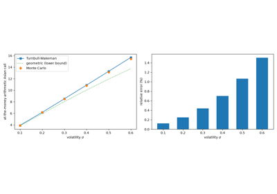
Stuart Turnbull and Lee Wakeman priced the arithmetic Asian option as if the average were lognormal with its exact first two moments. The moments are elementary integrals of \(E[S_t]\) and \(E[S_t S_u]\), and the option is Black’s formula on the mean of the average with the matched volatility. The approximation is excellent at moderate volatility and overprices as the average’s distribution grows more skewed than a lognormal. Edmond Levy’s 1992 version uses the exact discrete-fixing moments.

\[\sigma_A^2 = \frac{1}{T}\ln\frac{E[A^2]}{E[A]^2}, \qquad V = e^{-rT}\left[E[A] N(d_1) - K N(d_2)\right]\]

Implementation: financialkit.exotic_options.systems.asian.turnbull_wakeman_price() handles continuous averaging (the second moment by Gauss-Legendre quadrature, which stays accurate where the closed form cancels) and discrete fixings (Levy’s sums, in linear time). The example measures the approximation error against controlled Monte Carlo as volatility grows.

References: S. M. Turnbull and L. M. Wakeman, “A Quick Algorithm for Pricing European Average Options,” Journal of Financial and Quantitative Analysis 26 (1991) 377-389; E. Levy, “Pricing European Average Rate Currency Options,” Journal of International Money and Finance 11 (1992) 474-491.

Turnbull-Wakeman Asian approximation

1992 – Ikeda-Kunitomo Double Barriers #

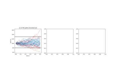
Naoto Ikeda and Masaaki Kunitomo priced options that knock out if the price leaves a corridor, even with exponentially curved boundaries. The transition density of Brownian motion killed at two barriers is an infinite series of images reflected alternately through both, and the option is a sum of Black-Scholes-like terms. The terms die off like \(e^{-2n^2 \ln^2(U/L)/\sigma^2 T}\), so a few suffice unless the corridor is narrow. A double knock-out call loses value as volatility rises.

\[c = S e^{(b-r)T}\sum_{n=-\infty}^{\infty}\left[\left(\tfrac{U^n}{L^n}\right)^{\mu}(N(d_1) - N(d_2)) - \left(\tfrac{L^{n+1}}{U^n S}\right)^{\mu}(N(d_3) - N(d_4))\right] - K e^{-rT}\sum_{n}[\dots]\]

Implementation: financialkit.exotic_options.systems.barriers.double_barrier_price() prices knock-out and knock-in calls and puts with flat barriers and a configurable number of terms. The example draws knocked-out paths, plots the value across the corridor for several volatilities and measures how fast the series converges.

References: N. Ikeda and M. Kunitomo, “Pricing Options with Curved Boundaries,” Mathematical Finance 2 (1992) 275-298; Haug (2007), Section 4.17.3.

Ikeda-Kunitomo double barriers

1992 – Reiner’s Quantos #

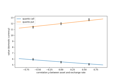
A quanto pays a foreign asset’s payoff in domestic currency at a rate fixed in advance, so an investor can hold the Nikkei without holding the yen. Eric Reiner showed that under the domestic risk-neutral measure the foreign asset’s drift picks up the covariance with the exchange rate, \(-\rho\sigma_S\sigma_X\), and the quanto is Black’s formula on the adjusted forward, discounted at the domestic rate. The correlation, not the level of the exchange rate, is what the seller is exposed to.

\[V = \bar X e^{-r_d T}\left[\hat F N(d_1) - K N(d_2)\right], \qquad \hat F = S e^{(r_f - q - \rho\sigma_S\sigma_X)T}\]

Implementation: financialkit.exotic_options.systems.multi_asset.quanto_price() calls financialkit.options.black76_price() on the adjusted forward. The example plots quanto calls and puts against the correlation and checks them with a Monte Carlo under the foreign measure.

References: E. Reiner, “Quanto Mechanics,” Risk 5(3) (1992) 59-63; Haug (2007), Section 5.16.

Reiner quantos

1997 – Broadie-Glasserman-Kou Discrete Barriers #

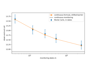
Barrier contracts check the price at the daily close, not continuously, and the continuous formulas overstate the chance of knocking out. Mark Broadie, Paul Glasserman and Steven Kou proved that a barrier monitored \(m\) times behaves like a continuous one moved away from the spot by \(e^{\beta\sigma\sqrt{T/m}}\), where \(\beta = -\zeta(1/2)/\sqrt{2\pi} \approx 0.5826\) comes from the expected overshoot of a Gaussian random walk. The correction removes the \(O(1/\sqrt m)\) error at no cost.

\[V_m(H) = V\!\left(H e^{\pm\beta\sigma\sqrt{T/m}}\right) + o(1/\sqrt m)\]

Implementation: financialkit.exotic_options.systems.barriers.discrete_barrier_price() applies the shift to barrier_price(), and BGK_BETA holds the constant. The example compares discretely monitored Monte Carlo with the shifted and the unshifted formulas from weekly to daily monitoring.

References: M. Broadie, P. Glasserman and S. Kou, “A Continuity Correction for Discrete Barrier Options,” Mathematical Finance 7 (1997) 325-349.

Broadie-Glasserman-Kou discrete barriers

1999 – Demeterfi-Derman-Kamal-Zou Variance Swaps #

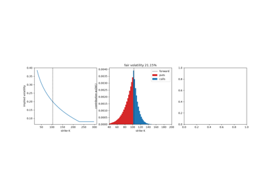
A variance swap pays realized variance against a fixed strike, a pure bet on volatility. Kresimir Demeterfi, Emanuel Derman, Michael Kamal and Joseph Zou showed that, for any continuous price process, it is replicated by a delta-hedged log contract, and the log contract by a static strip of out-of-the-money puts and calls weighted by \(1/K^2\). The fair strike is then read off today’s option prices, with no model of volatility at all. Discretised, the same sum became the CBOE’s VIX index in 2003.

\[K_{\mathrm{var}} = \frac{2e^{rT}}{T}\left[\int_0^{F}\frac{P(K)}{K^2}\,dK + \int_F^{\infty}\frac{C(K)}{K^2}\,dK\right]\]

Implementation: financialkit.exotic_options.systems.variance_swaps.variance_swap_strike() discretises the strip as in the VIX calculation and returns a VarianceSwapResult with each option’s weight, and realized_variance() computes the floating leg. The example shows the strip under a skew, which lifts the fair strike above the at-the-money volatility, and compares realized variance under Black-Scholes with the strike.

References: K. Demeterfi, E. Derman, M. Kamal and J. Zou, “A Guide to Volatility and Variance Swaps,” Journal of Derivatives 6(4) (1999) 9-32; Cboe, VIX White Paper (2003).

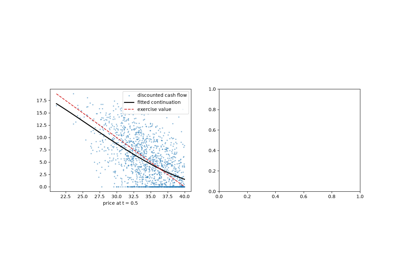
Demeterfi-Derman-Kamal-Zou variance swaps

2001 – Longstaff-Schwartz Least-Squares Monte Carlo #

Simulation runs forward in time, but early exercise is decided backward, and for twenty years American options seemed out of Monte Carlo’s reach. Francis Longstaff and Eduardo Schwartz estimated the value of continuing by regressing the realized discounted cash flows of the in-the-money paths on a few functions of the current price, and exercised each path where the payoff beats the fit. The method extends to many assets and to path-dependent payoffs, where trees and PDEs break down, and is now the standard way to price callable and Bermudan products by simulation.

\[\hat C(S_{t_i}) = \sum_{k} \beta_k \psi_k(S_{t_i}), \qquad \beta = \arg\min \sum_{\text{ITM paths}} \left(e^{-r\Delta t} Y_{t_{i+1}} - \sum_k \beta_k\psi_k(S_{t_i})\right)^2\]

Implementation: financialkit.exotic_options.systems.american.longstaff_schwartz() hand-writes the backward regression with weighted Laguerre or monomial regressors (regression_basis()) on paths from financialkit.integrators.gbm_paths(), and returns a LongstaffSchwartzResult with the exercise boundary. The example shows one regression step and compares the price and boundary with a binomial tree.

References: F. A. Longstaff and E. S. Schwartz, “Valuing American Options by Simulation: A Simple Least-Squares Approach,” Review of Financial Studies 14 (2001) 113-147; P. Glasserman, Monte Carlo Methods in Financial Engineering (Springer, 2004), Section 8.6.

Longstaff-Schwartz least-squares Monte Carlo