Breakthroughs in Market Microstructure#

financialkit.market_microstructure hub · History · Examples · API reference

“‘Market liquidity’ is a slippery and elusive concept, in part because it encompasses a number of transactional properties of markets.” – Albert Kyle (1985)

Asset-pricing theory takes prices as given; market microstructure asks how they are made. Someone has to stand ready to trade, and that service has a price: the bid-ask spread. Economists first explained it by the dealer’s costs and inventory risk, then, in 1985, by the realisation that some traders know more than others, which turned the order flow itself into information and the spread into insurance against it. The same ideas produced estimators of spreads and of informed trading that need nothing but prices or trade counts, and, once trading became electronic and algorithmic, models of how to execute a large order and how to make markets by machine. This chronology traces the ideas behind financialkit.market_microstructure.

1968 – Demsetz: The Cost of Transacting #

Harold Demsetz asked what investors pay to trade on the New York Stock Exchange beyond commissions. His answer was the bid-ask spread, the price of immediacy: a trader who will not wait for a counterparty pays a dealer to stand ready. In a cross-section of NYSE stocks the spread fell with the number of transactions, because a busy dealer turns over inventory faster. Modern practice measures it three ways, from quotes (quoted spread), from trades against the midquote (effective spread) and net of the subsequent price move (realized spread), the difference being the price impact that informed traders inflict.

\[s^{\text{eff}} = 2q(p - m_t) = \underbrace{2q(p - m_{t+\Delta})}_{\text{realized}} + \underbrace{2q(m_{t+\Delta} - m_t)}_{\text{impact}}\]

Implementation: financialkit.market_microstructure.systems.spreads.quoted_spread(), effective_spread(), realized_spread() and price_impact(). The example decomposes the effective spread of a simulated market and fits Demsetz’s spread-activity elasticity.

References: H. Demsetz, “The Cost of Transacting,” Quarterly J. Economics 82 (1968) 33-53; R. D. Huang and H. R. Stoll, “Dealer versus Auction Markets,” J. Financial Economics 41 (1996) 313-357.

Demsetz: the bid-ask spread as the price of immediacy

1976 – Garman’s Order-Flow Dealer #

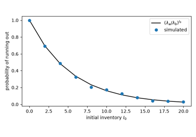
Mark Garman’s paper gave the field its name. Buyers and sellers arrive as Poisson streams whose rates depend on the ask and the bid, and a monopolist dealer clears them from its stock of shares and cash. The inventories are random walks, so the dealer fails with certainty unless both drift upward, which requires selling more dearly than it buys: the spread is the price of survival. The stock alone is a gambler’s-ruin problem with an explicit failure probability.

\[P(\text{run out of stock} \mid I_0) = \min\left(1, (\lambda_a / \lambda_b)^{I_0}\right)\]

Implementation: financialkit.market_microstructure.systems.dealers.garman_ruin_probability() and simulate_garman(). The example checks the ruin probability by simulation and shows dealers failing without a spread.

References: M. B. Garman, “Market Microstructure,” J. Financial Economics 3 (1976) 257-275; M. O’Hara, Market Microstructure Theory (Blackwell, 1995), Ch. 2.

Garman’s order-flow dealer

Garman's order-flow dealer

1981 – Ho and Stoll: Dealer Inventory Risk #

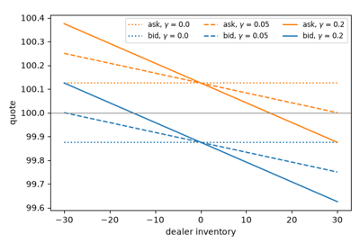
Thomas Ho and Hans Stoll made the dealer risk averse and the value of its inventory uncertain. A dealer who has bought too much now prefers selling to buying, so it lowers both quotes; one who is short raises them. The spread compensates for providing immediacy, while its position manages inventory. In a one-period mean-variance version with linear order arrival, the spread is independent of inventory and the midquote moves linearly against it.

\[\delta_a + \delta_b = \frac{\alpha}{\beta}, \qquad \frac{a + b}{2} = p - \frac{\gamma\sigma^2\tau\, I}{2(1 + \gamma\sigma^2\tau\beta)}\]

Implementation: financialkit.market_microstructure.systems.dealers.ho_stoll_quotes(). The example plots quotes against inventory for several risk aversions and simulates the resulting mean-reverting inventory.

References: T. Ho and H. R. Stoll, “Optimal Dealer Pricing under Transactions and Return Uncertainty,” J. Financial Economics 9 (1981) 47-73; H. R. Stoll, “The Supply of Dealer Services in Securities Markets,” J. Finance 33 (1978) 1133-1151.

Ho and Stoll: the dealer’s inventory problem

Ho and Stoll: the dealer's inventory problem

1984 – Roll’s Implicit Spread #

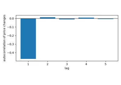
Richard Roll observed that if the value follows a random walk and each trade lands at the bid or the ask with equal probability, the bounce between them makes consecutive price changes negatively correlated, with first-order autocovariance \(-s^2/4\). The spread can therefore be estimated from transaction prices alone, which made it measurable for decades of daily data that has no quotes. In short samples the autocovariance is often positive, and the estimator is undefined.

\[\hat s = 2\sqrt{-\operatorname{cov}(\Delta p_t, \Delta p_{t-1})}\]

Implementation: financialkit.market_microstructure.systems.spreads.roll_spread(), using the autocovariance from financialkit.time_series.autocovariance(). The example shows the bounce in the autocorrelations and the estimator’s accuracy across spreads and sample sizes.

References: R. Roll, “A Simple Implicit Measure of the Effective Bid-Ask Spread in an Efficient Market,” J. Finance 39 (1984) 1127-1139.

Roll’s spread estimator

Roll's spread estimator

1985 – Kyle’s Insider #

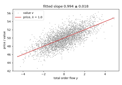
Albert Kyle modelled a single insider who knows the asset’s value, noise traders whose random orders give it cover, and a competitive market maker who sees only the total order flow. In the linear equilibrium the market maker moves the price by \(\lambda\) per unit of flow, a measure of the market’s depth known ever since as Kyle’s lambda, and the insider trades just enough that half of the private information is revealed. More noise trading makes the market deeper and the insider richer.

\[p = p_0 + \lambda(x + u), \qquad \lambda = \frac{\sigma_v}{2\sigma_u}, \qquad x = \frac{\sigma_u}{\sigma_v}(v - p_0)\]

Implementation: financialkit.market_microstructure.systems.information.kyle_equilibrium() and simulate_kyle(); kyle_lambda() estimates lambda by regression. The example recovers lambda from simulated auctions and shows that the equilibrium intensity maximises the insider’s profit.

References: A. S. Kyle, “Continuous Auctions and Insider Trading,” Econometrica 53 (1985) 1315-1335.

Kyle’s insider and the price impact lambda

Kyle's insider and the price impact lambda

1985 – Glosten and Milgrom: Adverse Selection #

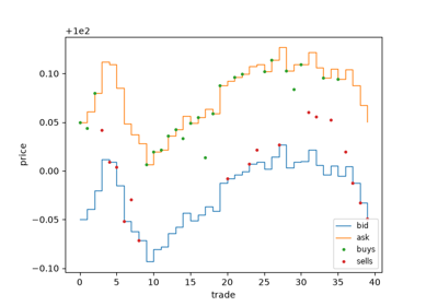
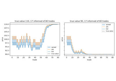
Lawrence Glosten and Paul Milgrom showed that a spread arises even when dealing is free and dealers are risk neutral. A buy order is more likely to come from someone who knows the value is high, so a competitive dealer sets the ask to the expected value given a buy and the bid to the expected value given a sell. The dealer loses to the informed what it earns from the uninformed, each trade updates its beliefs by Bayes’ rule, and the quotes converge to the true value.

\[a = E[V \mid \text{buy}], \qquad b = E[V \mid \text{sell}]\]

Implementation: financialkit.market_microstructure.systems.information.glosten_milgrom_quotes() and simulate_glosten_milgrom(). The example shows quotes converging on high and low values and the spread widening with the share of informed traders.

References: L. R. Glosten and P. R. Milgrom, “Bid, Ask and Transaction Prices in a Specialist Market with Heterogeneously Informed Traders,” J. Financial Economics 14 (1985) 71-100.

Glosten and Milgrom: a spread from adverse selection alone

1991 – Hasbrouck’s Trade-Impact VAR #

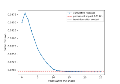
Joel Hasbrouck measured how much information trades carry with a vector autoregression of quote revisions and signed trades. Order flow is persistent and quotes also respond to inventory, so the immediate price reaction to a trade is a poor measure of its information. The cumulative response of the quote to an unexpected trade settles at the permanent impact, and the share of the efficient price’s variance that trade innovations explain says how much information arrives through trading rather than public news.

\[r_t = \sum_{i=1}^p a_i r_{t-i} + \sum_{i=0}^p b_i x_{t-i} + v_{1,t}, \qquad x_t = \sum_{i=1}^p c_i r_{t-i} + \sum_{i=1}^p d_i x_{t-i} + v_{2,t}\]

Implementation: financialkit.market_microstructure.systems.trade_impact.hasbrouck_var(), fitted with financialkit.time_series.utils.ols(). The example separates permanent from transitory impact in a market with persistent order flow and inventory effects.

References: J. Hasbrouck, “Measuring the Information Content of Stock Trades,” J. Finance 46 (1991) 179-207.

Hasbrouck’s trade-impact VAR

Hasbrouck's trade-impact VAR

1991 – Lee and Ready: Who Initiated the Trade?#

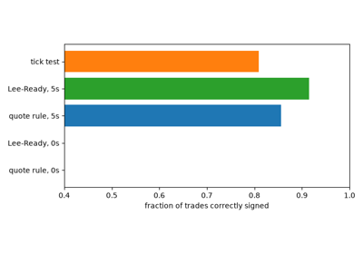
Spread, impact and informed-trading measures all need to know whether each trade was a buy or a sell, and trade records do not say. Charles Lee and Mark Ready combined the quote rule (above the midquote is a buy) with the tick test (an uptick is a buy) for trades exactly at the midquote, and compared each trade with the quote of five seconds earlier, because NYSE quote revisions triggered by a trade were often recorded before it. Their algorithm remains the default in empirical work.

Implementation: financialkit.market_microstructure.systems.classification.lee_ready(), tick_test() and quote_rule(), with financialkit.market_microstructure.utils.quotes.align_quotes() for the five-second rule. The example measures each rule’s accuracy with and without the delay.

References: C. M. C. Lee and M. J. Ready, “Inferring Trade Direction from Intraday Data,” J. Finance 46 (1991) 733-746.

Lee and Ready’s trade classification

Lee and Ready's trade classification

1996 – Easley, Kiefer, O’Hara and Paperman: PIN #

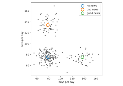
David Easley, Nicholas Kiefer, Maureen O’Hara and Joseph Paperman turned the Glosten-Milgrom model into something that could be estimated from daily counts of buys and sells. Each day news arrives with probability \(\alpha\); informed traders then add Poisson rate \(\mu\) to one side of a market where uninformed orders arrive at rates \(\varepsilon_b, \varepsilon_s\). Maximum likelihood on the resulting mixture gives the probability that a trade is informed, which they found higher in thinly traded stocks, explaining their wider spreads.

\[\mathrm{PIN} = \frac{\alpha\mu}{\alpha\mu + \varepsilon_b + \varepsilon_s}\]

Implementation: financialkit.market_microstructure.systems.informed_trading.fit_pin() maximises pin_loglik() with scipy.optimize.minimize() from several starting points and reports a delta-method standard error. The example fits simulated stocks of different activity.

References: D. Easley, N. M. Kiefer, M. O’Hara and J. B. Paperman, “Liquidity, Information, and Infrequently Traded Stocks,” J. Finance 51 (1996) 1405-1436.

Easley, Kiefer, O’Hara and Paperman: the probability of informed trading

Easley, Kiefer, O'Hara and Paperman: the probability of informed trading

1997 – The Square-Root Impact Law #

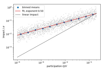
Executing a large order moves the price against the trader, and practitioners found that the impact of a whole metaorder grows like the square root of its size relative to daily volume, not linearly. Thomas Loeb’s 1983 cost tables showed the concave shape, and BARRA’s market impact model (Torre, 1997) put the square root into production. Later studies found it across markets, decades and asset classes, with an exponent close to one half; it is now among the most robust empirical regularities in finance.

\[I = Y\,\sigma\,\sqrt{Q / V}\]

Implementation: financialkit.market_microstructure.systems.execution.square_root_impact() and fit_impact_law(). The example fits the exponent to synthetic metaorders and compares with linear impact.

References: T. F. Loeb, “Trading Cost: The Critical Link between Investment Information and Results,” Financial Analysts J. 39 (1983) 39-44; N. Torre, BARRA Market Impact Model Handbook (BARRA, 1997); B. Tóth et al., “Anomalous Price Impact and the Critical Nature of Liquidity in Financial Markets,” Physical Review X 1 (2011) 021006.

The square-root impact law

1998 – Bertsimas and Lo: Optimal Control of Execution Costs #

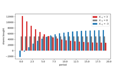
Dimitris Bertsimas and Andrew Lo posed best execution as stochastic dynamic programming. With a linear permanent price impact, a risk-neutral trader buying a block over several periods can do no better than an even split; when a serially correlated signal also moves prices, the optimal order is linear in the shares remaining and the latest signal, and the quadratic value function satisfies a simple backward recursion.

\[S_k = \left(1 - \frac{\theta}{2a_{k+1}}\right) W_k + \frac{\rho b_{k+1}}{2a_{k+1}} X_{k-1}\]

Implementation: financialkit.market_microstructure.systems.execution.bertsimas_lo(). The example recovers TWAP without information, shows the signal tilting the schedule and measures the saving by simulation.

References: D. Bertsimas and A. W. Lo, “Optimal Control of Execution Costs,” J. Financial Markets 1 (1998) 1-50.

Bertsimas and Lo: optimal control of execution costs

2000 – Almgren and Chriss: Efficient Execution #

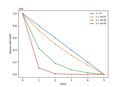
Robert Almgren and Neil Chriss separated permanent impact from the temporary impact of trading fast and added the trader’s aversion to the risk of holding the position. The optimal holdings decay as hyperbolic sines, from a straight line for a risk-neutral trader to near-immediate liquidation for a very risk-averse one, and sweeping the risk aversion traces an efficient frontier of expected cost against its variance. Their framework underlies most implementation-shortfall algorithms.

\[x_j = X\,\frac{\sinh(\kappa(T - t_j))}{\sinh(\kappa T)}, \qquad \cosh(\kappa\tau) = 1 + \frac{\lambda\sigma^2\tau^2}{2\tilde\eta}\]

Implementation: financialkit.market_microstructure.systems.execution.almgren_chriss() and execution_cost(). The example uses the paper’s worked example to draw trajectories and the efficient frontier.

References: R. Almgren and N. Chriss, “Optimal Execution of Portfolio Transactions,” J. Risk 3 (2000) 5-39.

Almgren and Chriss: the efficient frontier of execution

2002 – Amihud’s Illiquidity Ratio #

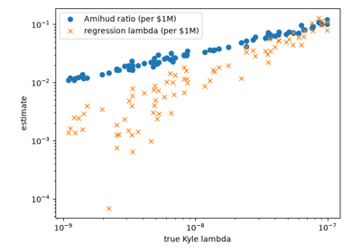
Yakov Amihud proposed measuring illiquidity as the average absolute daily return per dollar traded, a proxy for Kyle’s lambda that needs only daily returns and volume and so can be computed for every stock over long histories. He showed that expected returns rise with it, both across stocks and over time, an illiquidity premium. It remains the most widely used low-frequency liquidity measure.

\[\mathrm{ILLIQ} = \frac{1}{D}\sum_{d=1}^D \frac{|r_d|}{\mathrm{DVol}_d}\]

Implementation: financialkit.market_microstructure.systems.liquidity.amihud_illiquidity(). The example ranks a synthetic cross-section by Amihud’s ratio and compares it with the true and regression-estimated Kyle lambdas.

References: Y. Amihud, “Illiquidity and Stock Returns: Cross-Section and Time-Series Effects,” J. Financial Markets 5 (2002) 31-56.

Amihud’s illiquidity ratio

Amihud's illiquidity ratio

2008 – Avellaneda and Stoikov: Market Making in a Limit Order Book #

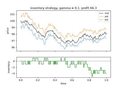
Marco Avellaneda and Sasha Stoikov wrote down the electronic market maker’s problem: quote around a mid price that moves as Brownian motion, get filled at a rate that decays exponentially with distance from the mid, and maximise exponential utility of terminal wealth. The solution first shifts the mid price to an inventory-adjusted reservation price and then sets an optimal spread around it, a continuous-time descendant of Ho and Stoll that became the template for algorithmic market making.

\[r = s - q\gamma\sigma^2(T - t), \qquad \delta_a + \delta_b = \gamma\sigma^2(T - t) + \frac{2}{\gamma}\ln\left(1 + \frac{\gamma}{k}\right)\]

Implementation: financialkit.market_microstructure.systems.dealers.AvellanedaStoikov, reservation_price(), avellaneda_stoikov_spread() and simulate_market_making(), whose mid price comes from financialkit.integrators.brownian_increments(). The example reproduces the paper’s comparison with symmetric quoting.

References: M. Avellaneda and S. Stoikov, “High-Frequency Trading in a Limit Order Book,” Quantitative Finance 8 (2008) 217-224.

Avellaneda and Stoikov: market making in a limit order book

2012 – Corwin and Schultz: Spreads from Highs and Lows #

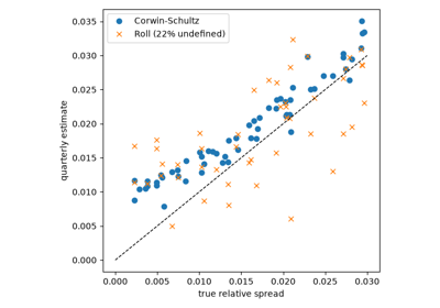
Shane Corwin and Paul Schultz noticed that daily highs are almost always buys at the ask and lows sells at the bid, so the high-low range contains both volatility and the spread. The volatility part of the squared log range doubles over two days while the spread part does not, so one two-day range and two one-day ranges identify the spread. The estimator needs only daily data and is far more accurate than Roll’s.

\[\alpha = \frac{\sqrt{2\beta} - \sqrt\beta}{3 - 2\sqrt2} - \sqrt{\frac{\gamma}{3 - 2\sqrt2}}, \qquad S = \frac{2(e^\alpha - 1)}{1 + e^\alpha}\]

Implementation: financialkit.market_microstructure.systems.spreads.corwin_schultz_spread(). The example compares monthly and quarterly estimates with the true spread and with Roll’s estimator from daily closes.

References: S. A. Corwin and P. Schultz, “A Simple Way to Estimate Bid-Ask Spreads from Daily High and Low Prices,” J. Finance 67 (2012) 719-760.

Corwin and Schultz’s high-low spread estimator

Corwin and Schultz's high-low spread estimator

2012 – Easley, López de Prado and O’Hara: VPIN #

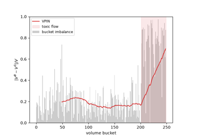
In high-frequency markets the PIN likelihood is impractical, and information arrives in volume rather than clock time. David Easley, Marcos López de Prado and Maureen O’Hara grouped trading into buckets of equal volume, split each bar’s volume into buys and sells by the standardised price change (bulk volume classification), and averaged the absolute order imbalance over recent buckets. Their measure of flow toxicity rose in the hours before the flash crash of 6 May 2010; its predictive power has been debated since.

\[\mathrm{VPIN} = \frac{1}{n}\sum_{\tau=1}^{n} \frac{|V^B_\tau - V^S_\tau|}{V}, \qquad V^B = V\,\Phi\left(\frac{\Delta P}{\sigma_{\Delta P}}\right)\]

Implementation: financialkit.market_microstructure.systems.informed_trading.vpin() and bulk_volume_classification(). The example tracks VPIN through a simulated episode of toxic selling.

References: D. Easley, M. M. López de Prado and M. O’Hara, “Flow Toxicity and Liquidity in a High-Frequency World,” Review of Financial Studies 25 (2012) 1457-1493; T. G. Andersen and O. Bondarenko, “VPIN and the Flash Crash,” J. Financial Markets 17 (2014) 1-46.

VPIN: flow toxicity in volume time