Breakthroughs in Credit Risk#

financialkit.credit hub · History · Examples · API reference

“Credit is a system whereby a person who can’t pay gets another person who can’t pay to guarantee that he can pay.” – Charles Dickens, Little Dorrit (1857)

For most of the twentieth century credit analysis meant reading financial statements and assigning a letter grade. In under four decades it became quantitative: statistics on accounting ratios, option pricing applied to the firm, Poisson processes for the timing of default, Markov chains for ratings, and factor models and copulas for whole portfolios, culminating in the formula that sets bank capital worldwide and the CDS conventions that still govern the market. This chronology traces the ideas behind financialkit.credit.

1968 – Altman’s Z-Score #

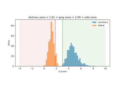
Edward Altman applied Fisher’s linear discriminant analysis to 22 accounting ratios of 66 US manufacturers, half of which had gone bankrupt, and kept the five that separated them best: liquidity, accumulated profitability, operating profitability, market leverage and asset turnover. The weighted sum classified 95% of his sample correctly a year before failure, and its thresholds of 1.81 and 2.99 are still quoted.

\[Z = 1.2 X_1 + 1.4 X_2 + 3.3 X_3 + 0.6 X_4 + 1.0 X_5\]

Implementation: financialkit.credit.systems.scoring.altman_z_score(), altman_zone() and linear_discriminant(). The example scores synthetic healthy and failing firms and re-estimates the discriminant direction.

References: E. I. Altman, “Financial Ratios, Discriminant Analysis and the Prediction of Corporate Bankruptcy,” J. Finance 23 (1968) 589-609.

Altman’s Z-score

Altman's Z-score

1974 – Merton’s Structural Model #

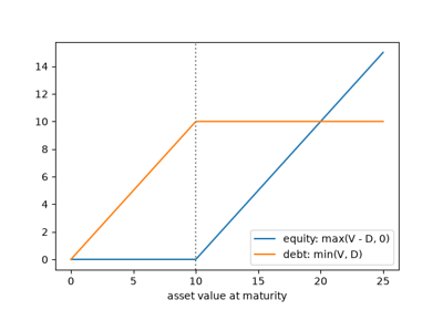
Robert Merton observed that the shareholders of a firm with zero-coupon debt hold a call option on its assets: at maturity they repay the debt if the assets are worth more, and hand over the firm otherwise. The Black-Scholes formula then values equity, debt and the credit spread from leverage and asset volatility alone, and the risk-neutral default probability is \(N(-d_2)\).

\[E = V N(d_1) - D e^{-rT} N(d_2), \qquad D_{\text{market}} = V - E\]

Implementation: financialkit.credit.systems.structural.merton_model() and merton_calibrate(), which recovers asset value and volatility from equity and its volatility (Hull’s Example 24.3). The example plots the payoffs and the term structure of Merton spreads.

References: R. C. Merton, “On the Pricing of Corporate Debt: The Risk Structure of Interest Rates,” J. Finance 29 (1974) 449-470.

Merton’s structural model

Merton's structural model

1976 – Black and Cox: First Passage #

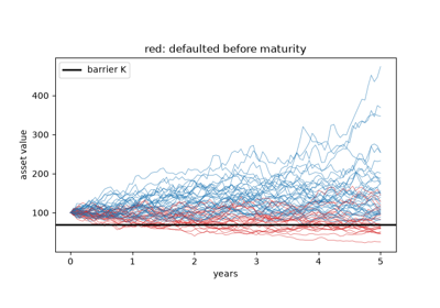
Fischer Black and John Cox let bond covenants trigger default the first time the assets fall to a barrier, at any date before maturity. Via the reflection principle for Brownian motion the default probability is again in closed form, and it is always at least the probability of ending below the barrier that Merton’s model uses.

\[Q(t) = N\left(\frac{h + m t}{\sigma\sqrt t}\right) - e^{-2 m h/\sigma^2} N\left(\frac{-h + m t}{\sigma\sqrt t}\right)\]

Implementation: financialkit.credit.systems.first_passage.black_cox_survival(), black_cox_default_probability() and the Brownian-bridge Monte Carlo check first_passage_crossing_probability(). The example compares the closed form with simulated asset paths and with Merton.

References: F. Black and J. C. Cox, “Valuing Corporate Securities: Some Effects of Bond Indenture Provisions,” J. Finance 31 (1976) 351-367.

Black and Cox: default at the first passage

1987 – Vasicek’s Large Homogeneous Portfolio #

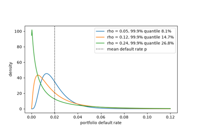
Oldrich Vasicek, at KMV, put Merton’s model into a portfolio. When every loan’s asset return loads on one common factor, defaults are independent given the factor, and in a large pool the default rate converges to a deterministic function of it. Its distribution has a closed form whose quantiles give the capital a lender needs, and the same formula sits inside the Basel II rules.

\[P(L \le x) = N\left(\frac{\sqrt{1-\rho}\, N^{-1}(x) - N^{-1}(p)}{\sqrt\rho}\right)\]

Implementation: financialkit.credit.systems.vasicek.vasicek_cdf(), vasicek_pdf(), vasicek_quantile() and simulate_one_factor_defaults(). The example shows the density for several correlations and finite pools converging to the limit.

References: O. Vasicek, “Probability of Loss on Loan Portfolio” (KMV, 1987); O. Vasicek, “The Distribution of Loan Portfolio Value,” Risk 15 (2002) 160-162.

Vasicek’s large homogeneous portfolio

Vasicek's large homogeneous portfolio

1994 – Leland’s Endogenous Default #

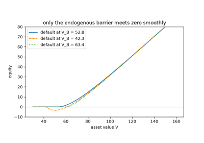
Hayne Leland priced perpetual debt when coupons are tax deductible and bankruptcy destroys part of the firm. Shareholders choose when to stop paying, so the default barrier is set by smooth pasting rather than by a covenant. Firm value trades the tax shield against expected bankruptcy costs, and its maximum gives an optimal leverage, about 75% with a 75 bp spread in Leland’s base case.

\[V_B = \frac{(1 - \tau) C}{r + \sigma^2/2}\]

Implementation: financialkit.credit.systems.leland.leland_model() and leland_optimal_coupon(). The example shows smooth pasting at the endogenous barrier and the capital-structure trade-off.

References: H. E. Leland, “Corporate Debt Value, Bond Covenants, and Optimal Capital Structure,” J. Finance 49 (1994) 1213-1252.

Leland’s endogenous default and optimal leverage

Leland's endogenous default and optimal leverage

1995 – Jarrow and Turnbull: Hazard Rates #

Robert Jarrow and Stuart Turnbull stopped asking why firms default and modelled only when: default is the first jump of a Poisson process. Survival probabilities are exponentials of the integrated intensity, risky bonds are priced like riskless ones with a survival factor, and spreads, hazard rates and recovery are linked by the credit triangle. These reduced-form models became the language of credit derivatives.

\[Q(t) = e^{-\int_0^t \lambda(s)\,ds}, \qquad P^d(0, T) = P(0, T)[\delta + (1 - \delta) Q(T)]\]

Implementation: financialkit.credit.systems.hazard.HazardCurve (piecewise-constant intensity, survival, density and sampling of default times) and jarrow_turnbull_zero(). The example simulates default times and compares bond spreads with the credit triangle.

References: R. A. Jarrow and S. M. Turnbull, “Pricing Derivatives on Financial Securities Subject to Credit Risk,” J. Finance 50 (1995) 53-85.

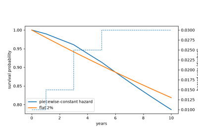
Jarrow and Turnbull: hazard rates and survival curves

1997 – CreditMetrics #

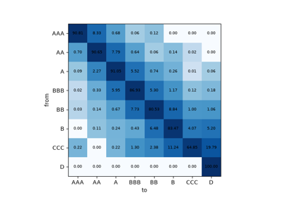
J. P. Morgan’s CreditMetrics did for credit what RiskMetrics had done for market risk. A bond is revalued in every rating it could migrate to over a year, the values are weighted with a rating agency’s transition matrix, and credit VaR is read from the distribution. Joint migrations come from correlated asset returns mapped to ratings by normal thresholds. The Technical Document’s five-year BBB bond has mean value 107.09 and standard deviation 2.99.

Implementation: financialkit.credit.systems.migration.creditmetrics_bond(), migration_thresholds(), joint_migration_probabilities() and creditmetrics_portfolio(), with the published matrix in creditmetrics_matrix(). The example reproduces the BBB bond and simulates a correlated portfolio.

References: J. P. Morgan, CreditMetrics – Technical Document (1997).

CreditMetrics: credit VaR from rating migrations

1997 – Jarrow, Lando and Turnbull: Generator Matrices #

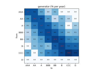
Robert Jarrow, David Lando and Stuart Turnbull moved rating migration to continuous time. A generator matrix of migration intensities gives the transition matrix for any horizon through the matrix exponential, so default probabilities and credit spreads exist for every maturity and every rating, and a risk-premium adjustment links historical and pricing measures.

\[P(t) = e^{\Lambda t}\]

Implementation: financialkit.credit.systems.migration.transition_from_generator() (scipy.linalg.expm()) and jlt_risky_zero(). The example plots default-probability term structures and spreads by rating.

References: R. A. Jarrow, D. Lando and S. M. Turnbull, “A Markov Model for the Term Structure of Credit Risk Spreads,” Rev. Financial Stud. 10 (1997) 481-523.

Jarrow, Lando and Turnbull: generator matrices

1997 – CreditRisk+ and Panjer’s Recursion #

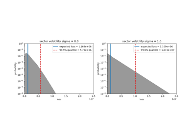
Credit Suisse First Boston brought actuarial science to loan portfolios. Defaults are Poisson events whose rates share a gamma-distributed sector factor, exposures are banded into integer loss units, and the loss distribution follows exactly from Panjer’s 1981 recursion for compound distributions, with no simulation at all.

\[f_n = \frac{1}{1 - a s_0} \sum_{j=1}^{n} \left(a + \frac{b j}{n}\right) s_j f_{n-j}\]

Implementation: financialkit.credit.systems.creditrisk_plus.creditrisk_plus() on top of panjer_recursion(). The example shows how sector volatility fattens the tail.

References: Credit Suisse First Boston, CreditRisk+: A Credit Risk Management Framework (1997); H. H. Panjer, “Recursive Evaluation of a Family of Compound Distributions,” ASTIN Bull. 12 (1981) 22-26.

CreditRisk+ and Panjer’s recursion

CreditRisk+ and Panjer's recursion

1999 – Duffie and Singleton: Recovery of Market Value #

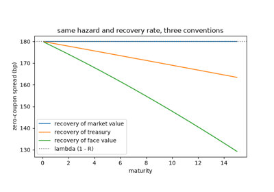
Darrell Duffie and Kenneth Singleton assumed that a defaulting claim loses a fraction of its own market value. Defaultable claims are then priced exactly like riskless ones under the default-adjusted short rate \(r + \lambda L\), so affine term-structure models price credit too, including stochastic intensities.

\[P^d(0, T) = E\left[e^{-\int_0^T (r_s + \lambda_s L)\,ds}\right]\]

Implementation: financialkit.credit.systems.recovery.risky_zero_coupon() (market value, treasury and face-value recovery) and duffie_singleton_cir_zero(). The example compares the conventions and checks the CIR closed form by simulation.

References: D. Duffie and K. J. Singleton, “Modeling Term Structures of Defaultable Bonds,” Rev. Financial Stud. 12 (1999) 687-720.

Duffie and Singleton: recovery of market value

2000 – Li’s Gaussian Copula #

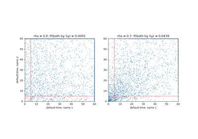
David Li joined default times with a Gaussian copula. Each name keeps the survival curve implied by its CDS spreads, and one correlation parameter controls how often names default together. The model priced basket swaps and CDOs for a decade, and its thin joint tail made it a symbol of the 2007-2008 crisis.

\[P(\tau_1 \le T, \tau_2 \le T) = \Phi_2\big(N^{-1}(p_1), N^{-1}(p_2); \rho\big)\]

Implementation: financialkit.credit.systems.copula_defaults.copula_default_times(), joint_default_probability(), default_correlation() and nth_to_default_probability(). The example shows joint default times and nth-to-default probabilities.

References: D. X. Li, “On Default Correlation: A Copula Function Approach,” J. Fixed Income 9 (2000) 43-54.

Li’s Gaussian copula for default times

Li's Gaussian copula for default times

2001 – Israel, Rosenthal and Wei: Finding Generators #

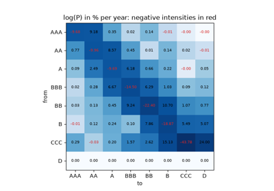
Agencies publish annual transition matrices, but continuous-time models need generators. Robert Israel, Jeffrey Rosenthal and Jason Wei showed that the matrix logarithm of an empirical rating matrix usually has negative off-diagonal entries, which would be negative migration intensities, gave conditions under which no valid generator exists, and proposed zeroing the offending entries and restoring the row sums.

Implementation: financialkit.credit.systems.migration.generator_from_transition() (scipy.linalg.logm()), is_valid_generator() and regularize_generator() (diagonal and weighted adjustments). The example regularizes the log of the CreditMetrics matrix and measures the error.

References: R. B. Israel, J. S. Rosenthal and J. Z. Wei, “Finding Generators for Markov Chains via Empirical Transition Matrices, with Applications to Credit Ratings,” Math. Finance 11 (2001) 245-265.

Israel, Rosenthal and Wei: finding a valid generator

2003 – Crosbie and Bohn: Distance to Default #

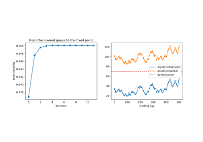
Moody’s KMV turned Merton’s model into a commercial default predictor. Peter Crosbie and Jeffrey Bohn described backing asset values out of a daily equity series by iteration, a default point of short-term debt plus half the long-term debt, and the distance to default, the number of standard deviations separating the two, mapped to an expected default frequency.

\[DD = \frac{\ln(V/D) + (\mu - \sigma_V^2/2) T}{\sigma_V \sqrt T}\]

Implementation: financialkit.credit.systems.structural.kmv_iterate(), kmv_default_point() and distance_to_default(). The example runs the iteration and a rolling distance to default.

References: P. J. Crosbie and J. R. Bohn, Modeling Default Risk (Moody’s KMV, 2003).

Crosbie and Bohn: the distance to default

2003 – O’Kane and Turnbull: The CDS Par Spread #

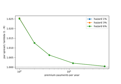
Dominic O’Kane and Stuart Turnbull set out the market-standard valuation of credit default swaps: the premium leg as a risky annuity including premium accrued at default, the protection leg as an integral over the default density, both evaluated on a grid with defaults at mid-step. The par spread equates them and reduces to \(\lambda(1 - R)\) in the continuous limit.

\[s = \frac{(1 - R)\int_0^T Z(u)\,(-dQ(u))}{\text{RPV01}}\]

Implementation: financialkit.credit.systems.cds.cds_legs() and cds_par_spread(). The example works Hull’s annual setting by hand and shows the approach to the credit triangle.

References: D. O’Kane and S. Turnbull, Valuation of Credit Default Swaps (Lehman Brothers, 2003).

O’Kane and Turnbull: the CDS par spread

O'Kane and Turnbull: the CDS par spread

2004 – The Basel II IRB Formula #

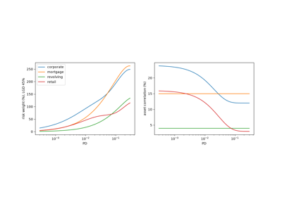
The Basel Committee’s revised framework let banks use their own default probabilities and set capital with Vasicek’s model at 99.9% confidence, less expected loss, times a maturity adjustment, with supervisory correlations by asset class. Michael Gordy had shown that this is the only setting in which a loan’s charge does not depend on the rest of the portfolio.

\[K = \left[LGD\, N\left(\frac{N^{-1}(PD) + \sqrt R N^{-1}(0.999)}{\sqrt{1 - R}}\right) - PD \cdot LGD\right] \frac{1 + (M - 2.5) b}{1 - 1.5 b}\]

Implementation: financialkit.credit.systems.basel.basel_irb_capital(), basel_risk_weight() and basel_correlation(). The example plots risk weights by asset class and the quantile behind them.

References: Basel Committee on Banking Supervision, International Convergence of Capital Measurement and Capital Standards: A Revised Framework (2004); M. B. Gordy, J. Financial Intermediation 12 (2003) 199-232.

The Basel II IRB formula

2004 – Hull and White: Tranches Without Monte Carlo #

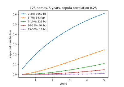
John Hull and Alan White priced CDO tranches and nth-to-default swaps in the one-factor copula semi-analytically: conditional on the factor, defaults are independent and the pool loss is binomial, so expected tranche losses at each payment date are a single integral. Correlation moves risk between the equity and senior tranches, which is why tranche quotes were read as implied correlations.

\[L_{[A, D]} = \frac{\min(L, D) - \min(L, A)}{D - A}\]

Implementation: financialkit.credit.systems.tranches.expected_tranche_loss() and tranche_spread(). The example shows tranche spreads against correlation and finite pools against the large-pool limit.

References: J. Hull and A. White, “Valuation of a CDO and an n-th to Default CDS Without Monte Carlo Simulation,” J. Derivatives 12 (2004) 8-23.

Hull and White: pricing CDO tranches without Monte Carlo

2009 – The ISDA Standard Model: Hazard Bootstrapping #

The 2009 “Big Bang” standardized CDS contracts: fixed coupons of 100 or 500 bp, an upfront payment, and an open-source ISDA standard model to convert between upfronts and spreads. Its core is a bootstrap of a piecewise-constant hazard curve, one maturity at a time, so that every quoted CDS reprices exactly.

Implementation: financialkit.credit.systems.cds.bootstrap_hazard_curve(), cds_upfront() and upfront_to_spread() (flat rate, even payment grid; ISDA day counts and IMM dates are not modelled). The example bootstraps a term structure of quotes and computes upfronts at both standard coupons.

References: ISDA, CDS Standard Model (2009); Markit, The CDS Big Bang (2009).

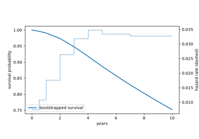
The ISDA standard model: bootstrapping hazard rates