Breakthroughs in Risk Measurement#

financialkit.risk hub · History · Examples · API reference

“VaR is like an airbag that works all the time, except when you have a car accident.” – David Einhorn (2008)

How much can a portfolio lose? For most of the twentieth century the answer was a standard deviation, which treats a windfall like a crash and says nothing about the worst days. Statisticians had meanwhile worked out the laws of extremes, of skewed quantiles and of dependence between variables, and in the 1990s banks and their regulators turned those results into value at risk, its backtests and, once its flaws were understood, expected shortfall. This chronology traces the ideas behind financialkit.risk.

1928 – Fisher and Tippett’s Extreme Value Laws #

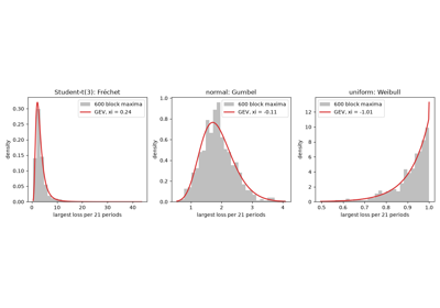
Ronald Fisher and Leonard Tippett asked what the largest of many independent observations looks like once centred and scaled. Only three limits are possible: the Fréchet law for power-law tails, the Gumbel law for exponential-type tails and the Weibull law for bounded ones. Boris Gnedenko made the result rigorous in 1943, and Jenkinson and von Mises folded the three into one family with a shape parameter \(\xi\). Fitting it to block maxima of losses, such as the worst day of each month, identifies the tail and extrapolates beyond the data.

\[H_\xi(x) = \exp\left(-(1 + \xi x)^{-1/\xi}\right), \qquad 1 + \xi x > 0\]

Implementation: financialkit.risk.systems.extreme_value.fit_gev() fits the GEV law to block maxima with scipy.stats.genextreme, and gev_return_level() gives the loss exceeded once every \(k\) blocks. The example fits Student-t, normal and uniform parents and compares return levels with the normal ones.

References: R. A. Fisher and L. H. C. Tippett, “Limiting Forms of the Frequency Distribution of the Largest or Smallest Member of a Sample,” Proc. Cambridge Phil. Soc. 24 (1928) 180-190; B. Gnedenko, Ann. Math. 44 (1943) 423-453.

Fisher-Tippett: the three laws of the maximum

1937 – The Cornish-Fisher Expansion #

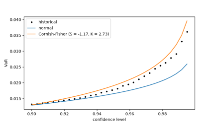
Edmund Cornish and Ronald Fisher expanded the quantile of a nearly normal distribution in its cumulants. To second order the correction needs only the skewness and the excess kurtosis. Sixty years later it became the standard way to adjust a parametric VaR for the negative skew and fat tails of returns, and of option books in delta-gamma approximations, at the cost of four sample moments.

\[z_{cf} = z + \frac{(z^2 - 1) S}{6} + \frac{(z^3 - 3z) K}{24} - \frac{(2z^3 - 5z) S^2}{36}\]

Implementation: financialkit.risk.systems.var.cornish_fisher_var() evaluates the expansion and broadcasts over confidence levels. The example compares it with exact quantiles of skewed distributions and with historical VaR on a skewed sample.

References: E. A. Cornish and R. A. Fisher, “Moments and Cumulants in the Specification of Distributions,” Rev. Int. Statist. Inst. 5 (1937) 307-320.

Cornish-Fisher: VaR beyond the normal

1952 – Roy’s Safety-First Criterion #

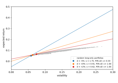
In the same year as Markowitz’s portfolio selection, Andrew Roy argued that investors care less about variance than about disaster: they want to minimise the probability that the return falls below a level \(d\). Knowing only means and variances, Chebyshev’s inequality bounds that probability by \(1/s^2\), so the safest portfolio maximises \(s = (\mu - d)/\sigma\). It was the first downside risk measure, and its ratio became the Sharpe ratio when \(d\) is the risk-free rate.

\[P(R < d) \le \frac{\sigma^2}{(\mu - d)^2} = \frac{1}{s^2}\]

Implementation: financialkit.risk.systems.safety_first.safety_first_ratio(), shortfall_probability() (Chebyshev or normal) and safety_first_portfolio(), the tangency portfolio from \(d\). The example draws Roy’s tangents for three disaster levels.

References: A. D. Roy, “Safety First and the Holding of Assets,” Econometrica 20 (1952) 431-449.

Roy’s safety-first criterion

Roy's safety-first criterion

1959 – Sklar’s Copulas #

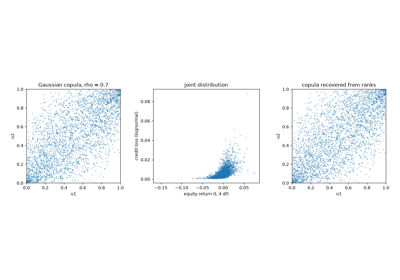
Answering a question of Maurice Fréchet, Abe Sklar proved that every joint distribution is its marginals coupled by a copula, a distribution on the unit cube with uniform marginals, and that the copula is unique when the marginals are continuous. Risk models could then choose each asset’s distribution separately from the dependence between them. The Gaussian copula, normal dependence under arbitrary marginals, became the industry default, for better and, in credit, for worse.

\[F(x_1, \ldots, x_d) = C\big(F_1(x_1), \ldots, F_d(x_d)\big)\]

Implementation: financialkit.risk.systems.copulas.gaussian_copula_sample() samples the Gaussian copula through financialkit.integrators.correlated_increments(), apply_marginals() performs Sklar’s construction, and financialkit.risk.utils.tail.pseudo_observations() recovers the copula from data by ranks. The example joins a Student-t equity return to a lognormal credit loss.

References: A. Sklar, “Fonctions de répartition à n dimensions et leurs marges,” Publ. Inst. Statist. Univ. Paris 8 (1959) 229-231.

Sklar’s theorem and the Gaussian copula

Sklar's theorem and the Gaussian copula

1975 – Pickands, Balkema and de Haan: Peaks Over Threshold #

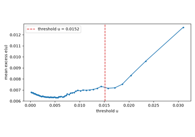
Block maxima waste data: a month with three crashes contributes one. James Pickands (1975), and independently August Balkema and Laurens de Haan (1974), proved that the excess of a loss over a high threshold is approximately generalized Pareto for every distribution in an extreme value domain. Fitting that law to all large losses, as McNeil and Frey did for VaR in 2000, gives tail quantiles and expected shortfall far beyond the empirical ones.

\[\mathrm{VaR}_\alpha = u + \frac{\beta}{\xi}\left[\left(\frac{n}{N_u}(1 - \alpha)\right)^{-\xi} - 1\right]\]

Implementation: financialkit.risk.systems.extreme_value.fit_pot() fits scipy.stats.genpareto to the exceedances, pot_var() and pot_es() extrapolate, and mean_excess() guides the choice of threshold. The example compares POT, historical and true VaR out to the 99.99% level.

References: J. Pickands, “Statistical Inference Using Extreme Order Statistics,” Ann. Statist. 3 (1975) 119-131; A. A. Balkema and L. de Haan, “Residual Life Time at Great Age,” Ann. Probab. 2 (1974) 792-804.

Peaks over threshold: Pickands-Balkema-de Haan

1991 – Young’s Calmar Ratio and Drawdowns #

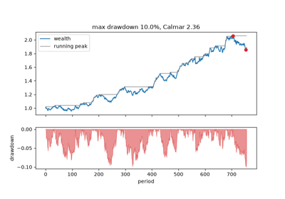
Terry Young, who published the California Managed Accounts Reports newsletter, proposed ranking commodity-trading advisors by their compound annual return over the last three years divided by their maximum drawdown. Drawdowns measure what investors actually live through, the fall from the best wealth reached so far, and they depend on the order of returns, which volatility ignores.

\[\text{Calmar} = \frac{\text{CAGR}}{\max_t \left(1 - W_t / \max_{s \le t} W_s\right)}\]

Implementation: financialkit.risk.systems.drawdowns.drawdowns() returns the drawdown path, its maximum, peak, trough and recovery, and calmar_ratio() the ratio. The example shows that reordering the same returns can multiply the drawdown.

References: T. W. Young, “Calmar Ratio: A Smoother Tool,” Futures 20(1) (1991) 40.

Young’s Calmar ratio and drawdowns

Young's Calmar ratio and drawdowns

1994 – RiskMetrics: Parametric VaR #

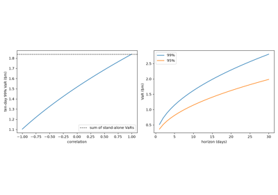
J.P. Morgan’s chairman Dennis Weatherstone wanted a single number, by 4:15 every afternoon, for how much the bank could lose the next day. The answer was value at risk under joint normality, and in October 1994 the bank published the method, RiskMetrics, and the covariance data to apply it, free. A whole trading book reduces to money exposures and a covariance matrix, and diversification appears explicitly.

\[\mathrm{VaR}_\alpha = z_\alpha \sqrt{h\, w^\top \Sigma w}\]

Implementation: financialkit.risk.systems.var.parametric_var() (normal or Student-t, with a horizon) and delta_normal_var() for portfolios. The example reproduces Hull’s Microsoft and AT&T example and the square-root-of-time rule.

References: J.P. Morgan/Reuters, RiskMetrics – Technical Document (1994; 4th ed. 1996); Hull, Options, Futures, and Other Derivatives, 10th ed., Ch. 22.

RiskMetrics: parametric (delta-normal) VaR

1995 – Kupiec’s Proportion-of-Failures Test #

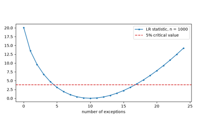
Once banks reported VaR, someone had to check it. Paul Kupiec, at the Federal Reserve Board, wrote the number of exceptions as a binomial variable and tested the observed rate against \(1 - \alpha\) by a likelihood ratio. His main finding was sobering: with a year of daily data the test can barely tell a correct 99% VaR from a badly wrong one.

\[LR_{uc} = -2 \ln \frac{(1 - p)^{n - x} p^x}{(1 - x/n)^{n - x} (x/n)^x} \sim \chi^2_1\]

Implementation: financialkit.risk.systems.backtesting.kupiec_test(), fed by financialkit.risk.utils.tail.var_exceptions(). The example tabulates the non-rejection regions and the test’s power against an understated volatility.

References: P. H. Kupiec, “Techniques for Verifying the Accuracy of Risk Measurement Models,” J. Derivatives 3(2) (1995) 73-84.

Kupiec’s proportion-of-failures test

Kupiec's proportion-of-failures test

1996 – Basel: Historical VaR and the Traffic Light #

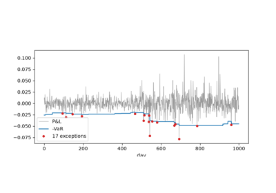
The Basel Committee’s Market Risk Amendment let banks compute capital from their own ten-day 99% VaR, estimated from at least a year of history, times a multiplier of at least 3. A companion document set the multiplier by backtesting: the binomial probability of the observed exceptions in 250 days puts a model in the green zone (0-4, no penalty), the yellow zone (5-9, plus 0.40 to 0.85) or the red zone (10 or more, plus 1). Historical simulation, which needs no distributional assumption, became the most common model.

\[\begin{split}\text{zone} = \begin{cases} \text{green} & P(X \le x) < 95\% \\ \text{red} & P(X \le x) \ge 99.99\% \\ \text{yellow} & \text{otherwise} \end{cases}, \quad X \sim \mathrm{Bin}(250, 0.01)\end{split}\]

Implementation: financialkit.risk.systems.var.historical_var(), rolling_historical_var() for out-of-sample forecasts, and financialkit.risk.systems.backtesting.basel_traffic_light(). The example runs a one-year historical VaR through a volatility jump and tracks its zone.

References: Basel Committee on Banking Supervision, Amendment to the Capital Accord to Incorporate Market Risks and Supervisory Framework for the Use of “Backtesting” (January 1996).

Basel historical VaR and the traffic light

1997 – Pritsker: Monte Carlo VaR #

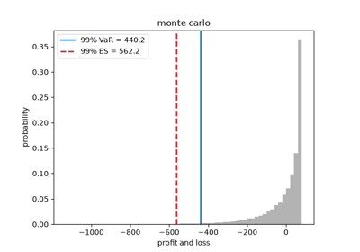
Matthew Pritsker compared the speed and accuracy of delta-normal, delta-gamma and full-revaluation Monte Carlo VaR on option portfolios. Linear and quadratic approximations failed exactly where options matter, for large moves and large gamma; full revaluation was accurate but expensive. For a delta-hedged short-volatility book the delta-normal VaR is zero while the true loss is large.

\[\mathrm{VaR}_\alpha = -\, Q_{1 - \alpha}\big(V(X_0 + \Delta X) - V(X_0)\big), \quad \Delta X \sim N(\mu h, \Sigma h)\]

Implementation: financialkit.risk.systems.var.monte_carlo_var() draws factor moves through financialkit.integrators.correlated_increments(), revalues with a user function, and reports an exact order-statistic confidence interval for the VaR. The example values short straddles with financialkit.options.black_scholes_price().

References: M. Pritsker, “Evaluating Value at Risk Methodologies: Accuracy versus Computational Time,” J. Financial Services Research 12 (1997) 201-242.

Pritsker: Monte Carlo VaR for option books

1998 – Boudoukh, Richardson and Whitelaw: Hybrid VaR #

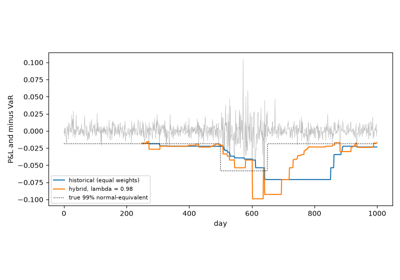
Historical simulation weights every day of its window equally, so it reacts slowly to a change in volatility and then jumps when an extreme day leaves the window. Jacob Boudoukh, Matthew Richardson and Robert Whitelaw weighted each past outcome by \(\lambda^i\), its age in days, and read the VaR off the weighted distribution: RiskMetrics’ exponential memory with historical simulation’s empirical tail.

\[P(\text{outcome } i \text{ days old}) = \frac{(1 - \lambda)\lambda^i}{1 - \lambda^n}\]

Implementation: financialkit.risk.systems.var.hybrid_var(), which is historical simulation for \(\lambda = 1\). The example compares the two through a turbulent spell.

References: J. Boudoukh, M. Richardson and R. Whitelaw, “The Best of Both Worlds,” Risk 11(5) (1998) 64-67.

Boudoukh-Richardson-Whitelaw hybrid VaR

1998 – Christoffersen’s Independence Test #

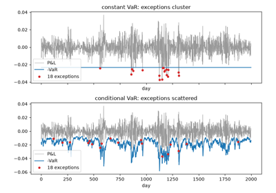
Peter Christoffersen pointed out that a VaR can have the right number of exceptions and still be useless if they all come in the same fortnight. He modelled the hit sequence as a two-state Markov chain and tested whether a hit is more likely after a hit; adding Kupiec’s statistic gave a joint test of conditional coverage.

\[LR_{ind} = -2 \ln \frac{(1 - \hat\pi)^{n_{00} + n_{10}} \hat\pi^{n_{01} + n_{11}}} {(1 - \hat\pi_{01})^{n_{00}} \hat\pi_{01}^{n_{01}} (1 - \hat\pi_{11})^{n_{10}} \hat\pi_{11}^{n_{11}}} \sim \chi^2_1\]

Implementation: financialkit.risk.systems.backtesting.christoffersen_independence() and christoffersen_test() (conditional coverage, \(\chi^2_2\)). The example backtests a constant and a GARCH VaR on a GARCH market.

References: P. F. Christoffersen, “Evaluating Interval Forecasts,” Int. Econ. Rev. 39 (1998) 841-862.

Christoffersen’s independence test

Christoffersen's independence test

1999 – Artzner, Delbaen, Eber and Heath: Coherent Risk Measures #

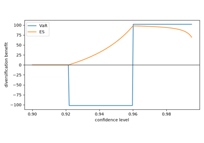
Philippe Artzner, Freddy Delbaen, Jean-Marc Eber and David Heath axiomatised what a capital requirement should be: monotone, subadditive, positively homogeneous and translation invariant. VaR fails subadditivity, so merging two portfolios can increase measured risk and splitting a bank can hide it. Two bonds that each default with probability 4% show it: each has a negative 95% VaR, their sum a large positive one.

\[\rho(X + Y) \le \rho(X) + \rho(Y)\]

Implementation: financialkit.risk.core.base.RiskMeasure, its subclasses financialkit.risk.systems.coherence.ValueAtRisk and ExpectedShortfall, and check_coherence(). The example reproduces the defaultable-bond counterexample across confidence levels.

References: P. Artzner, F. Delbaen, J.-M. Eber and D. Heath, “Coherent Measures of Risk,” Mathematical Finance 9 (1999) 203-228.

Artzner-Delbaen-Eber-Heath: coherent risk measures

1999 – Barone-Adesi: Filtered Historical Simulation #

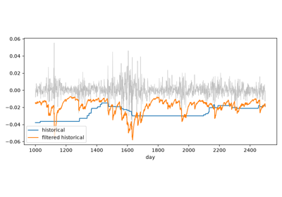
Giovanni Barone-Adesi, Kostas Giannopoulos and Les Vosper divided each historical return by its day’s GARCH volatility, giving standardized residuals that are close to i.i.d., and rescaled them by tomorrow’s forecast. The scenarios keep the empirical, fat-tailed shape of the shocks while their scale follows current market conditions, which removes most of plain historical simulation’s exception clustering.

\[\text{scenarios} = \hat\sigma_{n+1} \frac{r_t}{\sigma_t}, \qquad t = 1, \ldots, n\]

Implementation: financialkit.risk.systems.var.filtered_historical_var() accepts any volatility filter. The example estimates the filter with financialkit.time_series.GARCH, rolls filtered and plain historical VaR through a GARCH market with Student-t shocks, and backtests both.

References: G. Barone-Adesi, K. Giannopoulos and L. Vosper, “VaR without Correlations for Portfolios of Derivative Securities,” J. Futures Markets 19 (1999) 583-602.

Barone-Adesi: filtered historical simulation

1999 – Tasche: Euler Risk Allocation #

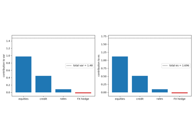
Dirk Tasche showed that for a risk measure that is homogeneous in the position sizes, the Euler contributions \(w_i\, \partial \rho / \partial w_i\) add up to the total and are the only allocation compatible with performance measurement: growing a position whose return on allocated capital beats the portfolio’s improves the portfolio. For VaR and ES on scenarios they are conditional expectations of each position’s loss given a portfolio loss in the tail.

\[\rho(w) = \sum_i w_i \frac{\partial \rho}{\partial w_i}(w)\]

Implementation: financialkit.risk.systems.allocation.euler_allocation() (normal volatility, VaR and ES) and scenario_es_allocation(). The example allocates a four-desk book with a short hedge, whose contribution is negative.

References: D. Tasche, “Risk Contributions and Performance Measurement,” working paper, Technische Universität München (1999).

Tasche: Euler risk allocation

2002 – Acerbi and Tasche: Expected Shortfall #

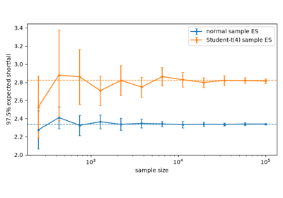
“Expected shortfall”, “conditional VaR”, “tail VaR” and “worst conditional expectation” were circulating as different definitions, some of them not coherent when the distribution has atoms, as every sample does. Carlo Acerbi and Dirk Tasche showed they coincide for continuous distributions and gave the general definition that is coherent: average exactly the worst fraction \(1 - \alpha\) of outcomes, with a partial weight on the quantile. In 2016 the Basel Committee’s Fundamental Review of the Trading Book replaced the 99% VaR by the 97.5% ES.

\[\mathrm{ES}_\alpha = -\frac{1}{1 - \alpha}\Big(E\big[X \mathbf{1}_{X < x_p}\big] + x_p\big(p - P(X < x_p)\big)\Big)\]

Implementation: financialkit.risk.systems.expected_shortfall.expected_shortfall(), built on financialkit.risk.utils.tail.weighted_tail(), which every scenario-based VaR in the subpackage shares, and the normal and Student-t closed forms parametric_es(). The example shows the estimator converging to both closed forms.

References: C. Acerbi and D. Tasche, “On the Coherence of Expected Shortfall,” J. Banking Finance 26 (2002) 1487-1503.

Acerbi-Tasche expected shortfall

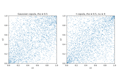
2005 – Demarta and McNeil: The t Copula #

The Gaussian copula has no tail dependence: however strong the correlation, joint extremes become independent far enough into the tail. Stefano Demarta and Alexander McNeil studied the t copula and its relatives, in which a common random scale makes crashes coincide, and gave its tail-dependence coefficient in closed form. It is positive even at zero correlation, which is why the t copula became the standard alternative for market and credit portfolios after 2008.

\[\lambda = 2\, t_{\nu + 1}\left(-\sqrt{\frac{(\nu + 1)(1 - \rho)}{1 + \rho}}\right)\]

Implementation: financialkit.risk.systems.copulas.t_copula_sample(), t_tail_dependence() and empirical_tail_dependence(). The example compares the corners of Gaussian and t copula samples with the same correlation.

References: S. Demarta and A. J. McNeil, “The t Copula and Related Copulas,” Int. Statist. Rev. 73 (2005) 111-129.

Demarta-McNeil: the t copula and tail dependence