Breakthroughs in Monte Carlo Methods#
“Anyone who considers arithmetical methods of producing random digits is, of course, in a state of sin.” – John von Neumann
Monte Carlo replaces an integral by an average over random samples. Its
error falls only like the inverse square root of the sample size, but
it falls that way in any dimension, which is why a method born in the
neutron-diffusion calculations at Los Alamos became the standard tool
for pricing path-dependent and multi-asset derivatives. Seventy years of
work have gone into making the square root hurt less: variance
reduction from survey statistics and operations research, quasi-random
points from number theory, Greeks without finite differences, and a
multilevel decomposition borrowed from multigrid solvers. This
chronology traces the ideas behind financialkit.monte_carlo.
1934 – Neyman Stratification#
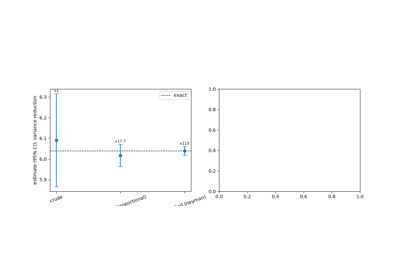
Jerzy Neyman’s paper to the Royal Statistical Society compared purposive selection with random sampling and settled the question in favour of stratified random samples. He also derived the allocation of a fixed sample between strata that minimises the variance of the estimated mean: proportional to each stratum’s weight times its standard deviation. Transplanted to simulation, the strata are pieces of the probability space of the driving random number, and the rule sends samples to where the payoff is most variable.
Implementation: financialkit.monte_carlo.systems.variance_reduction.stratified_estimate()
stratifies the uniform that drives a payoff into equal-probability
strata, with proportional allocation or Neyman’s allocation from a pilot
run (neyman_allocation()),
and returns a StratifiedResult.
The example prices an out-of-the-money call with both allocations.
References: J. Neyman, “On the Two Different Aspects of the Representative Method: The Method of Stratified Sampling and the Method of Purposive Selection,” Journal of the Royal Statistical Society 97 (1934) 558-625; P. Glasserman, Monte Carlo Methods in Financial Engineering (Springer, 2004), Section 4.3.
1949 – Metropolis-Ulam: the Monte Carlo Method#
Stanislaw Ulam’s idea of estimating the odds of solitaire by playing it, and John von Neumann’s plan to run the same experiment for neutrons on the ENIAC, were named and published by Nicholas Metropolis and Ulam in 1949. The paper set out the method’s two defining features: an integral or expectation is estimated by a sample mean, and the central limit theorem supplies the error bar, with a rate independent of the dimension.
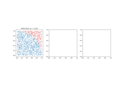
Implementation: financialkit.monte_carlo.systems.basics.monte_carlo_integrate()
returns a MonteCarloResult
with the standard error and a confidence interval; every other
estimator in the domain returns the same container. The example
estimates \(\pi\), ball volumes in two and six dimensions, and the
coverage of the 95% interval.
References: N. Metropolis and S. Ulam, “The Monte Carlo Method,” Journal of the American Statistical Association 44 (1949) 335-341; N. Metropolis, “The Beginning of the Monte Carlo Method,” Los Alamos Science 15 (1987) 125-130.
1953 – Kahn-Marshall Importance Sampling#
Herman Kahn and Andrew Marshall, at RAND, collected the variance reduction techniques then in use for radiation shielding, where almost no simulated particle penetrates the shield. Importance sampling draws from a different density that makes the important outcomes common and corrects with the likelihood ratio. They showed that the zero-variance density is proportional to the integrand itself, which is unusable but says what a good choice looks like. For normal drivers the natural family is a mean shift.
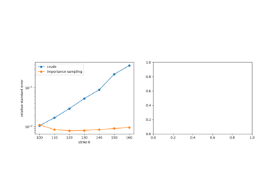
Implementation: financialkit.monte_carlo.systems.variance_reduction.importance_sampling_normal()
samples \(N(\theta, I)\) and applies the weight, for scalar or vector
shifts. The example prices deep out-of-the-money calls with the shift
that sends the stock to the strike, and scans the variance over the
shift.
References: H. Kahn and A. W. Marshall, “Methods of Reducing Sample Size in Monte Carlo Computations,” Journal of the Operations Research Society of America 1 (1953) 263-278; Glasserman (2004), Section 4.6.
1956 – Hammersley-Morton Antithetic Variates#
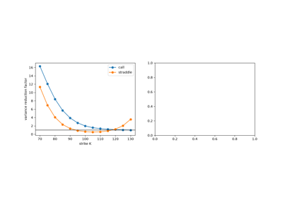
John Hammersley and Keith Morton proposed estimating an expectation from pairs of negatively correlated samples. For a uniform \(U\) the partner is \(1 - U\); for a normal it is \(-Z\). When the integrand is monotone the two halves of a pair err in opposite directions and the pair average has smaller variance than two independent draws; when it is symmetric the method backfires. It needs no knowledge of the problem and costs nothing, which has made it the default first step in derivatives pricing.
Implementation: financialkit.monte_carlo.systems.variance_reduction.antithetic_estimate()
averages mirrored pairs and takes the standard error over pairs; for
whole paths it pairs with financialkit.integrators.antithetic_increments().
The example contrasts a call (monotone, a gain) with a straddle (nearly
symmetric, a loss) and prices an Asian call on antithetic paths.
References: J. M. Hammersley and K. W. Morton, “A New Monte Carlo Technique: Antithetic Variates,” Mathematical Proceedings of the Cambridge Philosophical Society 52 (1956) 449-475; Glasserman (2004), Section 4.2.
1958 – Box-Muller Normal Variates#
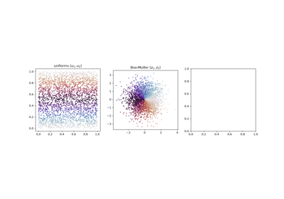
George Box and Mervin Muller published a two-paragraph note that solved the practical problem of turning a computer’s uniform random numbers into exact normal deviates. The joint density of two independent normals depends only on the radius, whose square is exponential, and the angle is uniform; inverting both distribution functions gives two normals from two uniforms with no rejection and no approximation.
Implementation: financialkit.monte_carlo.systems.basics.box_muller()
is the transform and box_muller_normals()
draws fresh normals with it. The example maps the uniform square to the
normal plane and checks the output with a Kolmogorov-Smirnov test.
References: G. E. P. Box and M. E. Muller, “A Note on the Generation of Random Normal Deviates,” Annals of Mathematical Statistics 29 (1958) 610-611.
1960 – Halton Sequences#
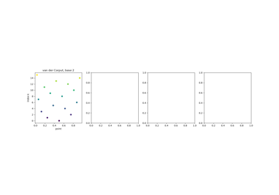
Johannes van der Corput had shown in 1935 that reversing the binary digits of the integers about the radix point gives a sequence that fills the unit interval with the smallest possible gaps. John Halton generalised it to the \(d\)-dimensional cube by using a different prime base in each coordinate, and proved that the resulting points integrate with an error of order \((\log N)^d / N\). The sequence is simple to compute and excellent in a handful of dimensions, but its projections onto pairs of large neighbouring primes are strongly correlated until the sample is very large.
Implementation: financialkit.monte_carlo.systems.quasi_monte_carlo.van_der_corput()
computes radical inverses directly and
halton() wraps
scipy.stats.qmc.Halton, optionally scrambled. The example shows
the gap-filling order, a correlated high-dimensional projection and the
integration error against random points.
References: J. H. Halton, “On the Efficiency of Certain Quasi-Random Sequences of Points in Evaluating Multi-Dimensional Integrals,” Numerische Mathematik 2 (1960) 84-90; J. G. van der Corput, “Verteilungsfunktionen,” Proc. Akad. Wet. Amsterdam 38 (1935) 813-821.
1961 – Koksma-Hlawka and Discrepancy#
Jurjen Koksma proved in 1942 that in one dimension the error of an equal-weight rule is at most the total variation of the integrand times the star discrepancy of the nodes; Edmund Hlawka extended the inequality to the cube in 1961, with the variation in the sense of Hardy and Krause. The bound separates the integrand from the points, explains why quasi-random points beat random ones, and defines the goal of the whole field: point sets of low discrepancy.
Implementation: financialkit.monte_carlo.systems.quasi_monte_carlo.star_discrepancy()
computes \(D_N^*\) exactly in one and two dimensions,
l2_star_discrepancy()
the \(L^2\) version in any dimension (via
scipy.stats.qmc.discrepancy()), and
koksma_hlawka_bound()
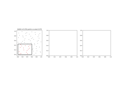
the bound. The example draws the local discrepancy of a box, compares
discrepancies of random, Halton and Sobol points, and checks the bound
for \(f(x, y) = xy\).
References: E. Hlawka, “Funktionen von beschränkter Variation in der Theorie der Gleichverteilung,” Annali di Matematica Pura ed Applicata 54 (1961) 325-333; J. F. Koksma, “Een algemeene stelling uit de theorie der gelijkmatige verdeeling modulo 1,” Mathematica B (Zutphen) 11 (1942) 7-11; H. Niederreiter, Random Number Generation and Quasi-Monte Carlo Methods (SIAM, 1992), Chapter 2.
1967 – Sobol Sequences#
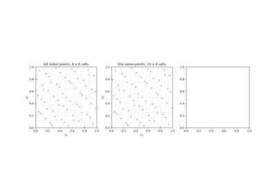
Ilya Sobol constructed base-2 digital sequences, generated by binary direction numbers, whose initial segments are nets: every dyadic box of the right volume contains exactly the right number of points. They are fast to generate with bitwise operations, remain well balanced in high dimension with good direction numbers, and became the default low-discrepancy sequence in finance after the 1990s.
Implementation: financialkit.monte_carlo.systems.quasi_monte_carlo.sobol()
wraps scipy.stats.qmc.Sobol (Joe-Kuo direction numbers). The
example verifies the net property on two grids and compares integration
errors with Halton and random points in eight dimensions.
References: I. M. Sobol, “On the Distribution of Points in a Cube and the Approximate Evaluation of Integrals,” USSR Computational Mathematics and Mathematical Physics 7 (1967) 86-112; S. Joe and F. Y. Kuo, “Constructing Sobol Sequences with Better Two-Dimensional Projections,” SIAM Journal on Scientific Computing 30 (2008) 2635-2654.
1977 – Boyle: Options by Monte Carlo#
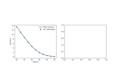
Four years after Black and Scholes, Phelim Boyle observed that risk-neutral valuation writes any European payoff’s price as a discounted expectation, so it can be simulated. He priced options on dividend-paying stocks, checked them against the closed form, used antithetic and control variates, and pointed out that the method handles payoffs and processes for which no formula exists. Simulation has been part of derivatives pricing ever since.
Implementation: financialkit.monte_carlo.systems.basics.european_option_mc()
simulates terminal prices through financialkit.integrators.gbm_paths()
and returns the price with its error bar. The example reproduces Hull’s
Example 15.6 and the price curve across strikes.
References: P. P. Boyle, “Options: A Monte Carlo Approach,” Journal of Financial Economics 4 (1977) 323-338; J. C. Hull, Options, Futures, and Other Derivatives, 10th ed. (Pearson, 2018), Chapter 21.
1979 – McKay-Beckman-Conover Latin Hypercube#
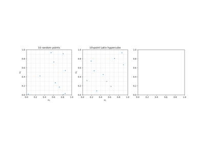
Michael McKay, Richard Beckman and William Conover, at Los Alamos, needed to explore the inputs of expensive computer models with few runs. Their Latin hypercube design places one point in each of \(n\) equal intervals of every coordinate, pairing the coordinates by independent random permutations, so that every one-dimensional margin is stratified simultaneously. They proved that the variance never exceeds crude Monte Carlo’s by more than a factor \(n/(n-1)\) for monotone integrands, and Stein (1987) showed that the additive part of the integrand is filtered out entirely.
Implementation: financialkit.monte_carlo.systems.variance_reduction.latin_hypercube_estimate()
uses scipy.stats.qmc.LatinHypercube and takes its standard
error from independent designs. The example shows the one-per-row,
one-per-column structure and prices a five-asset basket and a call on
it.
References: M. D. McKay, R. J. Beckman and W. J. Conover, “A Comparison of Three Methods for Selecting Values of Input Variables in the Analysis of Output from a Computer Code,” Technometrics 21 (1979) 239-245; M. Stein, “Large Sample Properties of Simulations Using Latin Hypercube Sampling,” Technometrics 29 (1987) 143-151.
1981 – Lavenberg-Welch Control Variates#
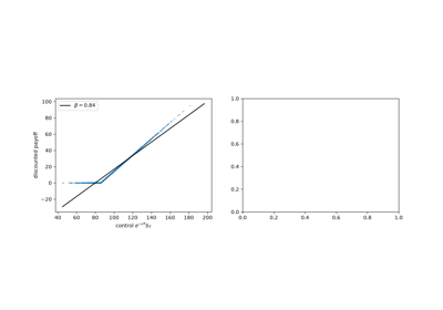
The idea of correcting a simulated mean by the observed error of a quantity with known expectation is old, but Stephen Lavenberg and Peter Welch gave it its modern form as a regression: the optimal coefficients are least-squares slopes, several controls can be used at once, and the variance falls by the fraction of variance the controls explain. In option pricing the discounted stock price, the geometric average of an Asian option or a simpler option with a closed form are all controls.
Implementation: financialkit.monte_carlo.systems.variance_reduction.control_variate_estimate()
fits \(\beta\) with numpy.linalg.lstsq() and returns a
ControlVariateResult with
the coefficients, \(R^2\) and the uncontrolled estimate. The example
draws the regression for a call on \(S_T\) and adds an at-the-money
call as a second control.
References: S. S. Lavenberg and P. D. Welch, “A Perspective on the Use of Control Variables to Increase the Efficiency of Monte Carlo Simulations,” Management Science 27 (1981) 322-335; Glasserman (2004), Section 4.1.
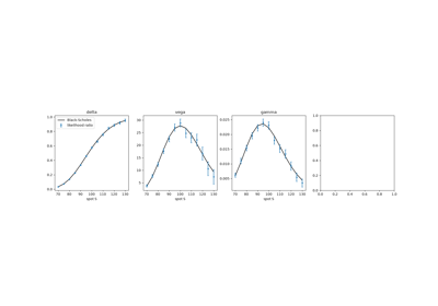
1987 – Glynn: Likelihood-Ratio Greeks#
Peter Glynn’s survey at the 1987 Winter Simulation Conference, and Reiman and Weiss’s paper of 1989, established the likelihood-ratio (or score-function) method for derivatives of expectations: differentiate the probability density of the simulated output rather than the output itself. The payoff is never differentiated, so discontinuous payoffs pose no problem; the price is a weight that grows noisier as the parameter’s influence spreads over more random inputs.
Implementation: financialkit.monte_carlo.systems.greeks.likelihood_ratio_greeks()
returns the price, delta, vega and gamma of vanilla or digital options
with standard errors in a
MonteCarloGreeks. The
example checks them against the Black-Scholes Greeks and the digital
call’s delta.
References: P. W. Glynn, “Likelihood Ratio Gradient Estimation: An Overview,” Proceedings of the 1987 Winter Simulation Conference, 366-375; M. I. Reiman and A. Weiss, “Sensitivity Analysis for Simulations via Likelihood Ratios,” Operations Research 37 (1989) 830-844; Glasserman (2004), Section 7.3.
1995 – Barraquand Moment Matching#
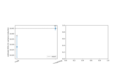
Jérôme Barraquand, valuing high-dimensional multivariate European securities, corrected the sampling error of the inputs directly: transform the sample of normals so that its mean and covariance are exactly the theoretical ones. “Quadratic resampling” makes simple moments of the payoff exact, at the cost of dependence between samples and an \(O(1/n)\) bias, so error bars must come from independent batches.
Implementation: financialkit.monte_carlo.systems.variance_reduction.moment_match()
rescales a sample and
moment_matching_estimate()
estimates with it over independent replications. The example compares
replicated crude and matched estimates of a call across sample sizes.
References: J. Barraquand, “Numerical Valuation of High Dimensional Multivariate European Securities,” Management Science 41 (1995) 1882-1891; Glasserman (2004), Section 4.5.
1995 – Owen Scrambling: Randomized QMC#
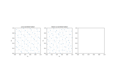
Quasi-Monte Carlo’s weakness was the missing error bar. Art Owen randomly permuted the base-\(b\) digits of a net in a nested way that preserves the net property: the scrambled points are still a net, yet each one is uniformly distributed. The estimate becomes unbiased, independent scramblings give a sample standard error, and Owen later proved that for smooth integrands the variance falls like \(N^{-3}(\log N)^{d-1}\), better than the unrandomized sequence.
Implementation: financialkit.monte_carlo.systems.quasi_monte_carlo.randomized_qmc_estimate()
integrates over independently scrambled Sobol or Halton point sets
(scipy.stats.qmc). The example shows that scrambling keeps the
stratification and that the root-mean-square error falls like
\(N^{-3/2}\).
References: A. B. Owen, “Randomly Permuted (t, m, s)-Nets and (t, s)-Sequences,” in Monte Carlo and Quasi-Monte Carlo Methods in Scientific Computing, Lecture Notes in Statistics 106 (Springer, 1995) 299-317; A. B. Owen, “Scrambled Net Variance for Integrals of Smooth Functions,” Annals of Statistics 25 (1997) 1541-1562.
1995 – Paskov-Traub: QMC in High Dimension#
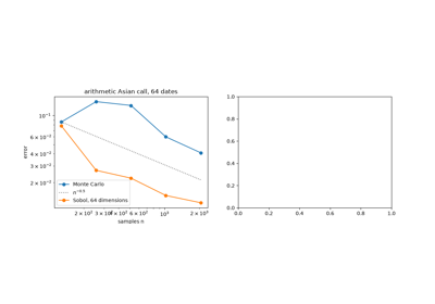
Conventional wisdom held that low-discrepancy sequences were useless beyond a few dozen dimensions. Spassimir Paskov and Joseph Traub valued a collateralized mortgage obligation from Goldman Sachs, a 360-dimensional integral, and found that Sobol points converged faster than Monte Carlo by a large factor. The resolution came from Caflisch, Morokoff and Owen’s notion of effective dimension: financial integrands are dominated by a few coordinates and low-order interactions, which the leading coordinates of a good sequence cover well.
Implementation: financialkit.monte_carlo.systems.quasi_monte_carlo.gbm_path_estimate()
prices a path-dependent payoff from pseudo-random or Sobol increments
(financialkit.integrators.sobol_increments(), time order), with
the standard error from replications. The example prices a 64-date
arithmetic Asian call and maps the payoff’s sensitivity to each
coordinate.
References: S. H. Paskov and J. F. Traub, “Faster Valuation of Financial Derivatives,” Journal of Portfolio Management 22 (1995) 113-120; R. E. Caflisch, W. Morokoff and A. Owen, “Valuation of Mortgage Backed Securities Using Brownian Bridges to Reduce Effective Dimension,” Journal of Computational Finance 1 (1997) 27-46.
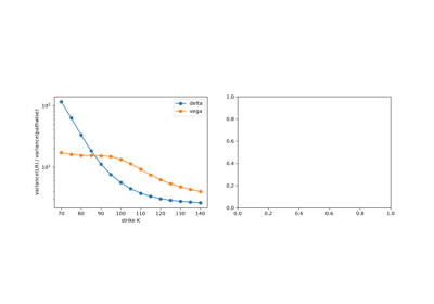
1996 – Broadie-Glasserman Pathwise Greeks#
Mark Broadie and Paul Glasserman set out two unbiased simulation estimators of price sensitivities side by side: the likelihood ratio and the pathwise derivative, which differentiates each simulated discounted payoff with respect to the parameter and averages. When the payoff is Lipschitz the derivative and the expectation commute, and the pathwise estimator is usually much less noisy; when the payoff jumps, as a digital does, it fails, and the two methods complement each other.
Implementation: financialkit.monte_carlo.systems.greeks.pathwise_greeks()
returns the pathwise delta and vega of a vanilla option (gamma is not
defined pathwise and is nan; digitals are refused). The example
compares its variance with the likelihood ratio on common random
numbers across strikes.
References: M. Broadie and P. Glasserman, “Estimating Security Price Derivatives Using Simulation,” Management Science 42 (1996) 269-285; Glasserman (2004), Section 7.2.
1996 – Caflisch-Moskowitz Brownian Bridge#
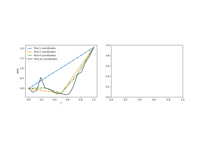
Russel Caflisch and Bradley Moskowitz, presenting quasi-Monte Carlo for finance at the 1994 Las Vegas conference (published 1995-96), proposed building each Brownian path by bisection: the first coordinate fixes the endpoint, the next the midpoint given the endpoints, and so on. The leading, best-distributed coordinates then carry most of the path’s variance, the effective dimension drops, and quasi-Monte Carlo gains substantially on path-dependent payoffs. Caflisch, Morokoff and Owen applied it to mortgage-backed securities in 1997.
Implementation: financialkit.integrators.brownian_bridge()
builds the paths and financialkit.monte_carlo.systems.quasi_monte_carlo.gbm_path_estimate()
with sampler="bridge" prices with them. The example shows the
coarse-to-fine construction and the gain over time-ordered Sobol points
on the 64-date Asian call.
References: R. E. Caflisch and B. Moskowitz, “Modified Monte Carlo Methods Using Quasi-Random Sequences,” in Monte Carlo and Quasi-Monte Carlo Methods in Scientific Computing, Lecture Notes in Statistics 106 (Springer, 1995) 1-16; W. J. Morokoff and R. E. Caflisch, “Quasi-Monte Carlo Integration,” Journal of Computational Physics 122 (1995) 218-230; Glasserman (2004), Section 5.5.
2008 – Giles Multilevel Monte Carlo#
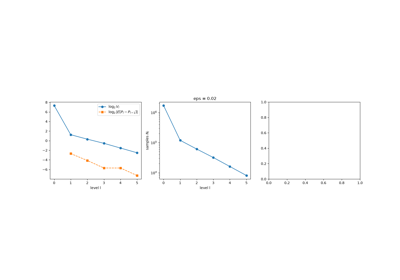
Michael Giles combined the telescoping idea of multigrid solvers and of Heinrich’s multilevel integration with SDE discretisation. The expectation on the finest grid is written as the coarsest expectation plus a sum of corrections, each estimated from fine and coarse Euler paths driven by the same Brownian increments. The corrections’ variance falls with the step size, so the optimal sample sizes decrease geometrically with the level, and the cost of a root-mean-square error \(\varepsilon\) falls from \(O(\varepsilon^{-3})\) to \(O(\varepsilon^{-2}(\log\varepsilon)^2)\). The idea has since spread to PDEs with random coefficients, nested simulation and Markov chain Monte Carlo.
Implementation: financialkit.monte_carlo.systems.multilevel.mlmc_level()
simulates coupled level corrections with
financialkit.integrators.euler_maruyama(), and
multilevel_monte_carlo()
runs Giles’s adaptive algorithm to a target accuracy, returning an
MLMCResult. The example
plots the level variances and sample sizes and the cost against
standard Monte Carlo.
References: M. B. Giles, “Multilevel Monte Carlo Path Simulation,” Operations Research 56 (2008) 607-617; M. B. Giles, “Multilevel Monte Carlo Methods,” Acta Numerica 24 (2015) 259-328; S. Heinrich, “Multilevel Monte Carlo Methods,” in Large-Scale Scientific Computing, LNCS 2179 (Springer, 2001) 58-67.