Breakthroughs in Asset Pricing#
“Asset pricing theory all stems from one simple concept, derived in the first page of the first chapter of this book: price equals expected discounted payoff.” – John H. Cochrane, Asset Pricing (2001)
What should an asset be worth, and why do some assets earn more than
others? The first answers were accounting ones: a share is worth the
dividends it will pay, discounted. Markowitz’s portfolio theory turned
the question into one about risk, and the capital asset pricing model
answered it with a single number, beta. Three decades of tests then
found the CAPM’s line too flat and its anomalies too many, and the field
moved to multifactor models built from the data itself. In parallel,
economists rebuilt the theory from the investor’s consumption and the
absence of arbitrage, arriving at one equation, \(p = E[m x]\),
whose discount factor \(m\) every model specifies differently, and
at puzzles that no simple specification of \(m\) resolves. This
chronology traces the ideas behind financialkit.asset_pricing.
1938 – Williams’s Dividend Discount Model#
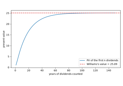
John Burr Williams’s Harvard dissertation, published as The Theory of Investment Value, defined a stock’s investment value as the present value of all its future dividends, with earnings mattering only through the dividends they fund. Williams built explicit forecasts of growth, payout and terminal value, and so wrote the first systematic manual of fundamental valuation, a decade before Graham and Dodd’s methods were codified as security analysis.
Implementation: financialkit.asset_pricing.systems.valuation.dividend_discount_value()
discounts explicit dividend forecasts and an optional Gordon terminal
value. The example shows how slowly the partial sums converge and how
much of the value lies beyond the forecast horizon.
References: J. B. Williams, The Theory of Investment Value, Harvard University Press (1938).
1958 – Modigliani and Miller#
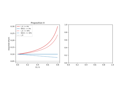
Franco Modigliani and Merton Miller argued by arbitrage that, in a frictionless market, two firms with the same operating cash flows must have the same total value however they are financed, since investors can lever or unlever on their own account (Proposition I). Debt is cheaper than equity, but borrowing makes the remaining equity riskier, and its expected return rises just enough to keep the average cost of capital constant (Proposition II). Their 1963 correction showed that the tax deductibility of interest adds a tax shield worth \(t D\). The arbitrage argument itself became the method of modern finance.
Implementation: financialkit.asset_pricing.systems.valuation.levered_cost_of_equity(),
wacc() and
levered_firm_value().
The example plots both propositions with and without corporate tax.
References: F. Modigliani and M. H. Miller, “The Cost of Capital, Corporation Finance and the Theory of Investment,” Am. Econ. Rev. 48 (1958) 261-297; “Corporate Income Taxes and the Cost of Capital: A Correction,” Am. Econ. Rev. 53 (1963) 433-443.
1959 – Gordon Growth#
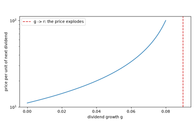
Myron Gordon summed Williams’s series for dividends that grow at a constant rate, giving the most widely used valuation formula in finance, and tied the growth rate to the firm’s investment: a firm that retains a fraction \(b\) of its earnings and earns a return \(ROE\) on them grows at \(b \cdot ROE\). Inverted, the formula gives the market’s cost of equity as the dividend yield plus growth, and it makes plain that retention creates value only when \(ROE\) exceeds \(r\).
Implementation: financialkit.asset_pricing.systems.valuation.gordon_growth_price()
calls financialkit.time_value.perpetuity_present_value(), with
implied_cost_of_equity()
and sustainable_growth().
The example shows the price’s explosion as \(g \to r\) and the value
of retention at different returns on equity.
References: M. J. Gordon, “Dividends, Earnings, and Stock Prices,” Rev. Econ. Statist. 41 (1959) 99-105.
1964 – Sharpe’s Capital Asset Pricing Model#
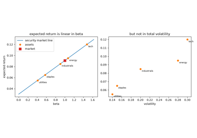
William Sharpe, and independently John Lintner (1965) and Jan Mossin (1966), asked what prices must be if every investor follows Markowitz. With a riskless asset, all investors hold the same tangency portfolio, which in equilibrium must be the market. The tangency condition prices every asset by its covariance with the market alone: risk that can be diversified away earns nothing. Sharpe shared the 1990 Nobel prize for it.
Implementation: financialkit.asset_pricing.systems.capm.capm_equilibrium()
finds the market as the tangency portfolio
(financialkit.risk.safety_first_portfolio()) and its betas;
capm_expected_return() and
estimate_beta(). The
example puts five sectors on the security market line and contrasts it
with total volatility.
References: W. F. Sharpe, “Capital Asset Prices: A Theory of Market Equilibrium under Conditions of Risk,” J. Finance 19 (1964) 425-442; J. Lintner, Rev. Econ. Statist. 47 (1965) 13-37.
1968 – Jensen’s Alpha#
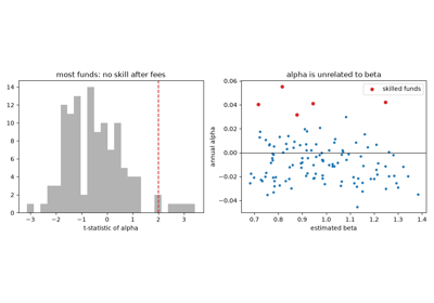
Michael Jensen turned the CAPM into a performance measure: regress a fund’s excess return on the market’s, and the intercept is the return earned beyond what its market risk justifies. Applied to 115 mutual funds from 1945 to 1964, it showed that the average fund underperformed by about the size of its fees, and that no more funds beat the market than chance would allow. The result fed directly into the efficient-markets view and, eventually, the index fund.
Implementation: financialkit.asset_pricing.systems.capm.jensen_alpha(),
the one-factor case of
time_series_regression().
The example simulates 115 funds, a handful of them skilled, and reads
their alphas and t-statistics.
References: M. C. Jensen, “The Performance of Mutual Funds in the Period 1945-1964,” J. Finance 23 (1968) 389-416.
1972 – Black’s Zero-Beta CAPM#
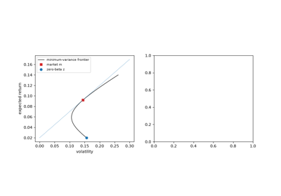
Fischer Black removed the CAPM’s least realistic assumption, unlimited borrowing at the riskless rate. Every portfolio on the minimum-variance frontier still prices all assets linearly in their betas on it, with the expected return of a zero-beta portfolio in place of the riskless rate. Because that return exceeds the lending rate, the security market line is flatter than Sharpe’s, which is what Black, Jensen and Scholes found in the data the same year.
Implementation: financialkit.asset_pricing.systems.capm.zero_beta_capm()
finds the frontier portfolio with a given zero-beta rate and the
minimum-variance portfolio uncorrelated with it. The example draws both
on the frontier and compares the two security market lines.
References: F. Black, “Capital Market Equilibrium with Restricted Borrowing,” J. Business 45 (1972) 444-455; F. Black, M. C. Jensen and M. Scholes, in Studies in the Theory of Capital Markets, Praeger (1972).
1973 – Fama-MacBeth Regressions#
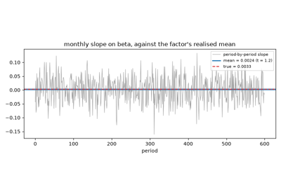
Eugene Fama and James MacBeth tested the CAPM with a cross-sectional regression of returns on betas each month, then averaged the slopes over time. The standard errors come from the time series of slopes, which handles the cross-correlation of returns without modelling it. Over 1935-1968 they found a positive price of beta, and no reward for beta squared or for idiosyncratic risk. The two-pass procedure is still the standard way to estimate factor risk premia.
Implementation: financialkit.asset_pricing.systems.factors.fama_macbeth()
runs both passes, or the second alone on given characteristics. The
example recovers a market premium and repeats Fama and MacBeth’s test
with beta squared and residual risk.
References: E. F. Fama and J. D. MacBeth, “Risk, Return, and Equilibrium: Empirical Tests,” J. Polit. Econ. 81 (1973) 607-636.
1976 – Ross’s Arbitrage Pricing Theory#
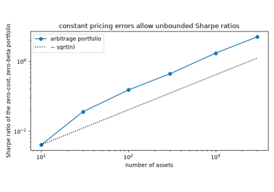
Stephen Ross derived linear pricing without assuming an equilibrium or mean-variance investors. If returns are driven by a few factors plus diversifiable noise, any asset off the plane \(E[r_i] = r_f + \beta_i'\lambda\) can be combined with others into a portfolio with no cost and no factor exposure that still earns a positive expected return. In a large market its risk diversifies away, so the pricing errors must be small for all but a few assets. The APT justified using several factors at once, and named none of them.
Implementation: financialkit.asset_pricing.systems.factors.apt_expected_returns()
and apt_arbitrage_portfolio(),
which builds the zero-cost, zero-beta portfolio from the residuals of
expected returns on the betas. The example shows its Sharpe ratio
growing without bound when pricing errors persist across many assets.
References: S. A. Ross, “The Arbitrage Theory of Capital Asset Pricing,” J. Econ. Theory 13 (1976) 341-360.
1978 – Lucas’s Tree#
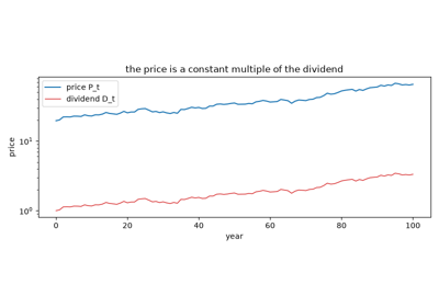
Robert Lucas priced assets in an exchange economy: a representative agent with power utility owns a tree whose fruit is the only consumption good, and prices must make the agent content to hold it. The Euler equation that results prices every asset with the discount factor \(\beta (C_{t+1}/C_t)^{-\gamma}\), and showed that a fully rational price can follow a random walk because the dividends it capitalises do. The model became the laboratory of consumption-based asset pricing.
Implementation: financialkit.asset_pricing.systems.consumption.LucasTree
prices the tree and the riskless bond in closed form for lognormal
growth and simulates the economy. The example shows the constant
price-dividend ratio and how rates and the premium vary with risk
aversion.
References: R. E. Lucas Jr., “Asset Prices in an Exchange Economy,” Econometrica 46 (1978) 1429-1445.
1979 – Harrison and Kreps: the Stochastic Discount Factor#
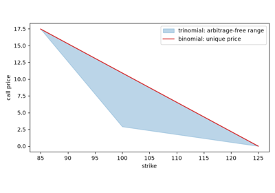
Michael Harrison and David Kreps proved that a market is free of arbitrage exactly when there is a strictly positive linear pricing rule consistent with every traded price: state prices, a positive discount factor, or an equivalent martingale measure, three forms of one object. Prices are unique when the market is complete; otherwise a new claim has an interval of arbitrage-free prices. This fundamental theorem made risk-neutral pricing rigorous and gave all of asset pricing the form \(p = E[m x]\).
Implementation: financialkit.asset_pricing.systems.sdf.FiniteStateMarket
finds positive state prices or an arbitrage portfolio with
scipy.optimize.linprog, and bounds the price of a new claim. The
example prices calls in complete binomial and incomplete trinomial
markets and exploits a mispriced stock.
References: J. M. Harrison and D. M. Kreps, “Martingales and Arbitrage in Multiperiod Securities Markets,” J. Econ. Theory 20 (1979) 381-408.
Harrison-Kreps: state prices and the stochastic discount factor
1979 – Breeden’s Consumption CAPM#
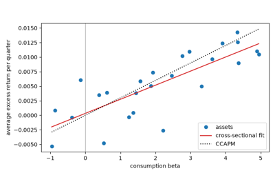
Merton’s intertemporal CAPM priced assets with one beta for every state variable that moves investment opportunities. Douglas Breeden showed that all of them collapse into a single beta on aggregate consumption: optimal consumption already responds to every state variable, so an asset’s premium is its covariance with consumption growth times risk aversion. Assets that pay off when consumption is low are insurance and earn less.
Implementation: financialkit.asset_pricing.systems.consumption.ccapm_expected_excess_return(),
with consumption betas from estimate_beta().
The example estimates the price of consumption risk from a
cross-section of assets and the implied risk aversion.
References: D. T. Breeden, “An Intertemporal Asset Pricing Model with Stochastic Consumption and Investment Opportunities,” J. Financ. Econ. 7 (1979) 265-296.
1981 – Shiller’s Excess Volatility#
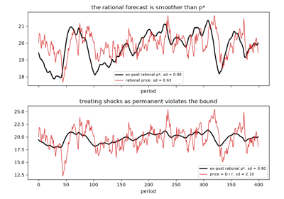
If prices are rational forecasts of discounted dividends, the price plus an unforecastable error equals the discounted value of the dividends actually paid. A forecast cannot vary more than what it forecasts, so prices must be less volatile than this ex-post rational price. Robert Shiller found US stock prices five to thirteen times too volatile, launching the debate over excess volatility that led to his 2013 Nobel prize and to the study of time-varying discount rates.
Implementation: financialkit.asset_pricing.systems.valuation.ex_post_rational_price(),
variance_bound() and
the AR(1) rational price
ar1_dividend_price().
The example shows a rational price respecting the bound and an
overreacting one violating it.
References: R. J. Shiller, “Do Stock Prices Move Too Much to be Justified by Subsequent Changes in Dividends?” Am. Econ. Rev. 71 (1981) 421-436.
1985 – Mehra and Prescott’s Equity Premium Puzzle#
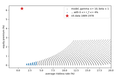
Rajnish Mehra and Edward Prescott calibrated a two-state Markov version of Lucas’s economy to US consumption from 1889 to 1978 and asked how large an equity premium it could produce. With risk aversion up to ten and a riskless rate below four percent, the answer was 0.35 percent, against 6.18 percent in the data. Consumption is too smooth for stocks to be that risky to a power-utility investor. Habit formation, recursive utility, rare disasters and long-run risks are all attempts to resolve the puzzle.
Implementation: financialkit.asset_pricing.systems.consumption.MehraPrescott
solves the price-dividend ratios and moments of the economy, and
implied_risk_aversion()
gives the risk aversion a premium requires. The example maps the
admissible region of riskless rates and premia against the data.
References: R. Mehra and E. C. Prescott, “The Equity Premium: A Puzzle,” J. Monet. Econ. 15 (1985) 145-161.
1989 – The Gibbons-Ross-Shanken Test#
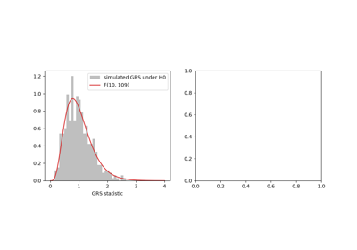
Testing the CAPM means asking whether the market portfolio is mean-variance efficient, or equivalently whether the time-series alphas of all test assets are jointly zero. Michael Gibbons, Stephen Ross and Jay Shanken gave the exact finite-sample F-distribution of that test under normal errors, and showed that it measures how much the tangency portfolio’s squared Sharpe ratio improves when the test assets join the factors. It remains the standard test of any traded factor model.
Implementation: financialkit.asset_pricing.systems.capm.grs_test().
The example checks the test’s size against the F-distribution and
traces its power against mispricing.
References: M. R. Gibbons, S. A. Ross and J. Shanken, “A Test of the Efficiency of a Given Portfolio,” Econometrica 57 (1989) 1121-1152.
1991 – The Hansen-Jagannathan Bound#
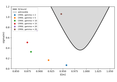
Lars Peter Hansen and Ravi Jagannathan asked what asset returns alone reveal about the discount factor. Any \(m\) that prices the returns must be volatile enough: \(\sigma(m)/E(m)\) is at least the highest Sharpe ratio available, and the full bound for each mean is attained by a combination of the returns themselves. With an equity Sharpe ratio near 0.4 a year, the power-utility discount factor enters the admissible region only at implausible risk aversion. Any candidate model can be screened against the bound before it is estimated.
Implementation: financialkit.asset_pricing.systems.sdf.hansen_jagannathan_bound()
and max_sharpe_ratio(). The
example draws the bound for stocks and bills and the moments of the
CRRA discount factor for increasing risk aversion.
References: L. P. Hansen and R. Jagannathan, “Implications of Security Market Data for Models of Dynamic Economies,” J. Polit. Econ. 99 (1991) 225-262.
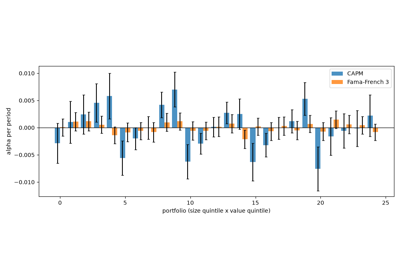
1993 – The Fama-French Three Factors#
By the early 1990s the CAPM had failed on two simple characteristics: small stocks and stocks with high book-to-market ratios earned more than their betas implied. Eugene Fama and Kenneth French built two long-short factors from the same sorts, SMB and HML, and showed that with the market they explained the returns of 25 size and value portfolios, leaving alphas near zero. The three-factor model replaced the CAPM as the benchmark for performance evaluation and empirical work.
Implementation: financialkit.asset_pricing.utils.sorts.long_short_factor()
and sort_portfolios()
build the factors and test portfolios, and
time_series_regression()
estimates the alphas. The example compares CAPM and three-factor
alphas of 25 synthetic size-value portfolios, with GRS tests.
References: E. F. Fama and K. R. French, “Common Risk Factors in the Returns on Stocks and Bonds,” J. Financ. Econ. 33 (1993) 3-56.
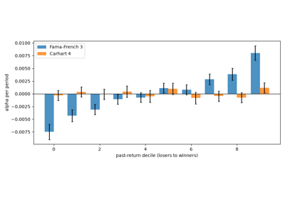
1997 – Carhart’s Momentum Factor#
Narasimhan Jegadeesh and Sheridan Titman (1993) showed that stocks with the best returns over the past year keep outperforming for months, an anomaly the three factors could not absorb. Mark Carhart added a fourth factor, UMD, long last year’s winners and short its losers, and used it to show that most persistence in mutual fund performance came from funds that happened to hold winning stocks rather than from skill. The four-factor model became the standard for fund evaluation.
Implementation: financialkit.asset_pricing.utils.sorts.momentum_signal()
computes the twelve-month, skip-one-month formation return, and
long_short_factor() turns
it into UMD. The example prices momentum deciles with three and four
factors.
References: M. M. Carhart, “On Persistence in Mutual Fund Performance,” J. Finance 52 (1997) 57-82; N. Jegadeesh and S. Titman, J. Finance 48 (1993) 65-91.