Breakthroughs in Financial Time Series#

financialkit.time_series hub · History · Examples · API reference

“The series looks like a wandering one, almost as if once a week the Demon of Chance drew a random number from a symmetrical population of fixed dispersion and added it to the current price to determine the next week’s price.” – Maurice Kendall, 1953

A price series is a single realization of a random process that can never be rerun, so everything known about it has to be inferred from its own past. Financial time-series analysis began by borrowing the autoregressions that statisticians had built for sunspots and rivers, and then found that prices broke their assumptions one by one. Prices wander like random walks, so their changes, not their levels, are the object of study. The changes are nearly uncorrelated, which is the efficient-markets hypothesis in statistical form, and much of the history is a sequence of ever sharper tests of that claim. Yet the changes are not independent: their size clusters, their tails are fat, and volatility responds more to falls than to rises. Two Nobel prizes, Engle’s and Granger’s in 2003, went to modelling these features. This chronology traces the ideas behind financialkit.time_series.

1927 – Yule’s Autoregression #

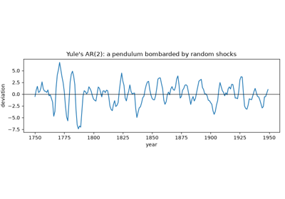
The standard tool for periodic data was Schuster’s periodogram, which treats a series as exact sine waves plus measurement error. Udny Yule found it unconvincing for sunspot numbers, whose cycles vary in length and height. He proposed instead a pendulum “bombarded by peas”: a damped oscillation that random shocks keep alive. For Wolfer’s sunspot numbers he fitted \(x_t = 1.34\,x_{t-1} - 0.65\,x_{t-2} + \varepsilon_t\), whose complex characteristic roots give a pseudo-cycle of about ten and a half years. The coefficients solve the Yule-Walker equations, a Toeplitz system in the sample autocorrelations. With this paper the autoregressive model, the backbone of time-series analysis, was born.

\[\rho_k = \sum_{i=1}^{p}\phi_i\,\rho_{k-i}, \quad k = 1, \dots, p\]

Implementation: financialkit.time_series.systems.linear_models.yule_walker() (via scipy.linalg.solve_toeplitz()), with ar_cycle_period() for the pseudo-period and simulate_arma().

References: G. U. Yule, “On a Method of Investigating Periodicities in Disturbed Series, with Special Reference to Wolfer’s Sunspot Numbers,” Philosophical Transactions of the Royal Society A 226 (1927) 267-298.

Yule’s autoregression

Yule's autoregression

1951 – Hurst Exponent #

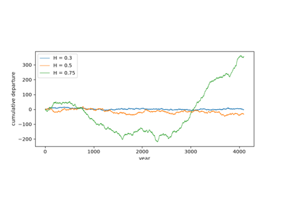
Harold Edwin Hurst spent decades measuring the Nile to size the reservoirs above Aswan. The storage a dam needs to release the average flow every year is the range \(R\) of cumulative departures from the mean. Divided by the standard deviation \(S\), this rescaled range grows like \(n^{1/2}\) for independent inflows, but Hurst found \(n^{0.73}\) for the Nile and for hundreds of other natural records. Wet years cluster with wet years over long horizons. Mandelbrot later explained the exponent \(H\) with fractional Brownian motion and brought it to finance, where \(H \ne 1/2\) would mean long-range predictability. Anis and Lloyd’s (1976) exact expectation of \(R/S\) for independent data corrects the estimate’s small-sample bias.

\[E\Bigl[\frac{R}{S}\Bigr]_n \propto n^{H}\]

Implementation: financialkit.time_series.systems.long_memory.hurst_exponent() returns a HurstResult with the raw and Anis-Lloyd-corrected exponents; simulate_fgn() generates exact fractional Gaussian noise by circulant embedding (scipy.fft).

References: H. E. Hurst, “Long-Term Storage Capacity of Reservoirs,” Transactions of the American Society of Civil Engineers 116 (1951) 770-799; A. A. Anis and E. H. Lloyd, “The Expected Value of the Adjusted Rescaled Hurst Range of Independent Normal Summands,” Biometrika 63(1) (1976) 111-116; B. B. Mandelbrot and J. W. Van Ness, “Fractional Brownian Motions, Fractional Noises and Applications,” SIAM Review 10(4) (1968) 422-437.

Hurst exponent

1953 – Kendall: the Random Walk of Prices #

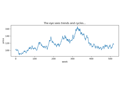
Maurice Kendall went looking for cycles in 22 British price series: wheat, cotton and industrial share indices, sampled weekly. Instead he found that the serial correlations of the price changes were close to zero at every lag, while the levels were almost perfectly correlated. He concluded that prices wander like a random walk. The finding surprised economists who had expected cycles, but it established the empirical fact that efficient-markets theory would explain a decade later: in a well-functioning market, past price changes do not predict future ones.

\[\hat\rho_k = \frac{\sum_{t}(x_t - \bar x)(x_{t-k} - \bar x)}{\sum_t (x_t - \bar x)^2}, \qquad |\hat\rho_k| \lesssim \frac{1.96}{\sqrt n}\ \text{under independence}\]

Implementation: financialkit.time_series.systems.efficiency.autocorrelation() (by FFT) and bartlett_band(); plot_acf() draws the correlogram.

References: M. G. Kendall, “The Analysis of Economic Time-Series – Part I: Prices,” Journal of the Royal Statistical Society A 116(1) (1953) 11-34.

Kendall: the random walk of prices

1963 – Mandelbrot: Fat Tails #

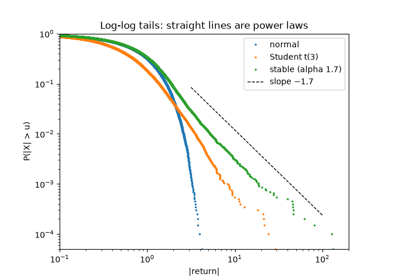
Benoit Mandelbrot plotted the frequency of large daily and monthly changes in cotton prices on doubly logarithmic paper and found straight lines. The tails decay like a power law, not like the Gaussian that Bachelier’s random walk assumed, so extreme moves are vastly more common than the normal distribution predicts. He proposed the stable Paretian laws, with index \(\alpha \approx 1.7\), which have infinite variance. He also noted that large changes tend to be followed by large changes. Later work settled on tail indices between 3 and 5 for most assets, so variances are finite, but fat tails and volatility clustering became the first two stylized facts of returns.

\[P(|X| > u) \sim C\,u^{-\alpha}, \qquad u \to \infty\]

Implementation: financialkit.time_series.systems.stylized_facts.tail_survival() (the log-log tail), return_statistics() (moments and the Jarque-Bera test via scipy.stats.jarque_bera()) and log_returns().

References: B. Mandelbrot, “The Variation of Certain Speculative Prices,” Journal of Business 36(4) (1963) 394-419; R. Cont, “Empirical Properties of Asset Returns: Stylized Facts and Statistical Issues,” Quantitative Finance 1(2) (2001) 223-236.

Mandelbrot: fat tails

1965 – Fama’s Runs Test #

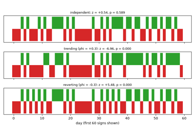
Eugene Fama’s thesis, published in full in the Journal of Business, examined the daily prices of the 30 Dow Jones Industrials. Correlation coefficients can be dominated by a few huge changes, which Mandelbrot had just shown to be common. Fama therefore added a distribution-free test that uses only the signs of the changes, counting the runs of consecutive changes with the same sign. Trends would produce too few runs and reversals too many. The counts were close to their expected values under independence. The paper, and Fama’s 1970 survey, made the efficient-markets hypothesis the organizing idea of empirical finance.

\[m = \frac{N(N+1) - \sum_i n_i^2}{N}, \qquad \sigma_m^2 = \frac{\sum_i n_i^2\bigl[\sum_i n_i^2 + N(N+1)\bigr] - 2N\sum_i n_i^3 - N^3}{N^2(N-1)}\]

Implementation: financialkit.time_series.systems.efficiency.runs_test() with Fama’s three-sign (+, -, 0) moments, returning a TestResult.

References: E. F. Fama, “The Behavior of Stock-Market Prices,” Journal of Business 38(1) (1965) 34-105; A. Wald and J. Wolfowitz, “On a Test Whether Two Samples Are from the Same Population,” Annals of Mathematical Statistics 11(2) (1940) 147-162.

Fama’s runs test

Fama's runs test

1970 – Box-Jenkins ARMA #

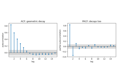
George Box and Gwilym Jenkins’s book turned mixed autoregressive moving-average models into a practical method with three stages. First, identify the orders from the autocorrelation function, which cuts off after lag \(q\) for a moving average, and the partial autocorrelation function, which cuts off after lag \(p\) for an autoregression. Second, estimate by maximum likelihood. Third, check the residuals for leftover structure, and repeat until they are white noise. Then forecast, with error bands from the model’s moving-average representation. ARMA models became the benchmark that every economic forecast had to beat.

\[\phi(B)(x_t - \mu) = \theta(B)\,\varepsilon_t, \qquad \operatorname{Var}(\hat x_{T+h} - x_{T+h}) = \sigma^2\sum_{j<h}\psi_j^2\]

Implementation: financialkit.time_series.systems.linear_models.fit_arma() (conditional maximum likelihood by scipy.optimize.least_squares(), kept stationary and invertible by Monahan’s transform), returning an ARMAResult with forecast(); partial_autocorrelation() (Durbin-Levinson), arma_acf() and arma_psi_weights().

References: G. E. P. Box and G. M. Jenkins, Time Series Analysis: Forecasting and Control (San Francisco: Holden-Day, 1970); J. F. Monahan, “A Note on Enforcing Stationarity in Autoregressive-Moving Average Models,” Biometrika 71(2) (1984) 403-404.

Box-Jenkins ARMA

1974 – Akaike Information Criterion #

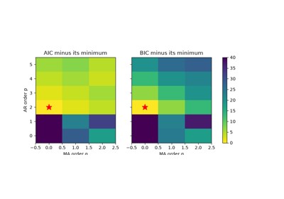
Box and Jenkins chose orders by inspecting correlograms. Hirotugu Akaike replaced the judgement call with a number. The maximized log-likelihood is an optimistic estimate of how well a model will predict new data, and Akaike showed that the optimism is about one unit per estimated parameter. Minimizing \(-2\ell + 2k\) therefore picks the model with the smallest expected Kullback-Leibler distance from the truth. Gideon Schwarz (1978) derived the heavier Bayesian penalty \(k \ln n\), which selects the true order with probability tending to one. AIC is better for prediction and BIC for identification.

\[\mathrm{AIC} = -2\ell(\hat\theta) + 2k, \qquad \mathrm{BIC} = -2\ell(\hat\theta) + k\ln n\]

Implementation: financialkit.time_series.systems.linear_models.select_arma_order() fits every order on a common sample and returns an OrderSelectionResult; every ARMAResult and VolatilityFit reports aic and bic.

References: H. Akaike, “A New Look at the Statistical Model Identification,” IEEE Transactions on Automatic Control 19(6) (1974) 716-723; G. Schwarz, “Estimating the Dimension of a Model,” Annals of Statistics 6(2) (1978) 461-464.

Akaike information criterion

1975 – Hill Tail Index #

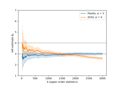
If a tail is a power law, the logarithms of the largest observations, measured from a high threshold, are exponentially distributed with mean \(1/\alpha\). Bruce Hill turned this into a simple estimator that uses only the \(k\) largest order statistics and is the maximum likelihood estimator for an exact Pareto tail. The Hill plot of \(\hat\alpha_k\) against \(k\) shows the central difficulty of tail estimation: small \(k\) is noisy, and large \(k\) reaches into the body of the distribution and is biased. Applied to returns, it gave tail indices between 3 and 5, so variances exist but fourth moments barely do.

\[\hat\alpha_k = \Bigl[\frac1k\sum_{i=1}^{k}\ln X_{(i)} - \ln X_{(k+1)}\Bigr]^{-1}, \qquad \operatorname{se}(\hat\alpha_k) \approx \frac{\alpha}{\sqrt k}\]

Implementation: financialkit.time_series.systems.stylized_facts.hill_estimator() returns a TailIndexResult for either tail; plot_hill() draws the Hill plot.

References: B. M. Hill, “A Simple General Approach to Inference About the Tail of a Distribution,” Annals of Statistics 3(5) (1975) 1163-1174.

Hill tail index

1978 – Ljung-Box Portmanteau Test #

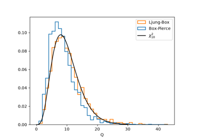
Checking many autocorrelations one by one is bound to find a “significant” one by chance. Box and Pierce (1970) pooled the first \(h\) into a single chi-squared statistic for diagnosing fitted ARMA residuals. Its distribution is far from \(\chi^2\) in samples of realistic size, so it rejected too rarely. Greta Ljung and George Box weighted each term by \((n+2)/(n-k)\), the reciprocal of its exact variance factor, and the corrected statistic matches its reference closely. Applied to squared returns rather than returns, the same test became a standard check for volatility clustering.

\[Q = n(n+2)\sum_{k=1}^{h}\frac{\hat\rho_k^2}{n-k} \;\sim\; \chi^2_{h-p-q}\]

Implementation: financialkit.time_series.systems.efficiency.ljung_box() and box_pierce(), with fitted_params for ARMA residuals.

References: G. M. Ljung and G. E. P. Box, “On a Measure of Lack of Fit in Time Series Models,” Biometrika 65(2) (1978) 297-303; G. E. P. Box and D. A. Pierce, “Distribution of Residual Autocorrelations in Autoregressive-Integrated Moving Average Time Series Models,” Journal of the American Statistical Association 65(332) (1970) 1509-1526.

Ljung-Box portmanteau test

1979 – Dickey-Fuller Unit Roots #

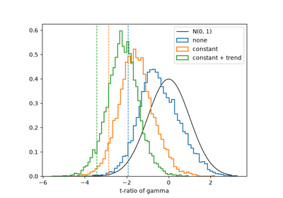
Whether a series has a unit root decides whether shocks to it are permanent, as for a stock price, or fade away, as for a stationary interest rate. The obvious test, the t-ratio of \(\gamma\) in \(\Delta y_t = \gamma y_{t-1} + e_t\), does not have a t distribution when \(\gamma = 0\): it is skewed to the left. David Dickey and Wayne Fuller derived and tabulated its distribution by simulation. Said and Dickey (1984) added lagged differences to absorb serial correlation, and James MacKinnon’s response surfaces give critical values for any sample size. Nelson and Plosser’s (1982) finding that most macroeconomic series cannot reject a unit root changed empirical macroeconomics.

\[\Delta y_t = \alpha + \beta t + \gamma y_{t-1} + \sum_{i=1}^{k}\delta_i\,\Delta y_{t-i} + e_t, \qquad H_0: \gamma = 0\]

Implementation: financialkit.time_series.systems.unit_roots.adf_test() (AIC lag selection), returning a UnitRootResult with mackinnon_critical_values(); simulate_dickey_fuller() traces the null distribution.

References: D. A. Dickey and W. A. Fuller, “Distribution of the Estimators for Autoregressive Time Series with a Unit Root,” Journal of the American Statistical Association 74(366) (1979) 427-431; S. E. Said and D. A. Dickey, “Testing for Unit Roots in Autoregressive-Moving Average Models of Unknown Order,” Biometrika 71(3) (1984) 599-607; J. G. MacKinnon, “Critical Values for Cointegration Tests,” Queen’s Economics Department Working Paper 1227 (2010).

Dickey-Fuller unit roots

1980 – Parkinson’s Range Volatility #

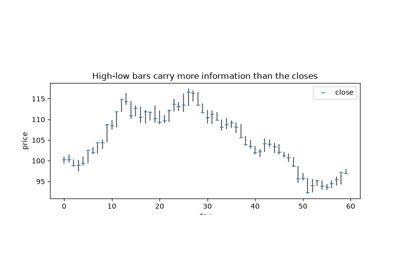
Close-to-close returns throw away almost everything that happened during the day. Michael Parkinson, a physicist, applied the theory of the range of Brownian motion. The squared log ratio of the high to the low, divided by \(4\ln 2\), is an unbiased estimate of the period’s variance and is about five times more efficient than the squared return. A month of daily ranges carries roughly as much information as five months of closes. The idea led to the Garman-Klass and Rogers-Satchell estimators and to range-based volatility models.

\[\hat\sigma^2_t = \frac{(\ln H_t - \ln L_t)^2}{4\ln 2}\]

Implementation: financialkit.time_series.systems.realized.parkinson_variance() and close_to_close_variance(); simulate_ohlc() builds daily bars from exact GBM paths (financialkit.integrators.gbm_paths()).

References: M. Parkinson, “The Extreme Value Method for Estimating the Variance of the Rate of Return,” Journal of Business 53(1) (1980) 61-65.

Parkinson’s range volatility

Parkinson's range volatility

1982 – Engle’s ARCH #

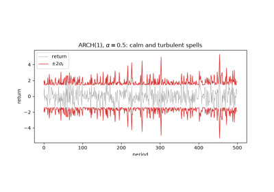
Robert Engle was modelling UK inflation, whose forecast errors were small in some periods and large in others. He let the conditional variance depend on past squared errors. The model’s returns are uncorrelated but not independent, cluster in volatility and have fat tails even with normal innovations, which reproduces Mandelbrot’s two stylized facts at once. Engle also gave a Lagrange-multiplier test that regresses squared residuals on their own lags. ARCH opened the econometrics of risk and earned him the 2003 Nobel prize.

\[r_t = \sigma_t z_t, \qquad \sigma_t^2 = \omega + \alpha\,r_{t-1}^2, \qquad \mathrm{LM} = T R^2 \sim \chi^2_q\]

Implementation: financialkit.time_series.systems.garch.ARCH (a VolatilityModel fitted by maximum likelihood) and arch_lm_test().

References: R. F. Engle, “Autoregressive Conditional Heteroscedasticity with Estimates of the Variance of United Kingdom Inflation,” Econometrica 50(4) (1982) 987-1007.

Engle’s ARCH

Engle's ARCH

1986 – Bollerslev’s GARCH #

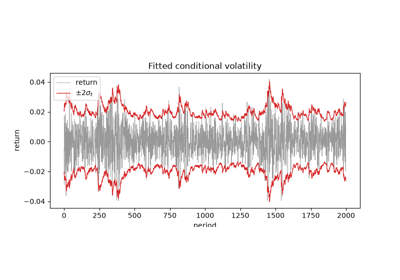
Volatility decays slowly, so pure ARCH needed long lag lists with awkward constraints. Tim Bollerslev, Engle’s student, added the lagged conditional variance itself, which gives an ARCH(\(\infty\)) with geometrically declining weights in just three parameters. GARCH(1,1) fitted to daily returns almost anywhere gives a small \(\alpha\) and a persistence \(\alpha + \beta\) just below one. It is still the default volatility model of practitioners, and its forecasts mean-revert to a long-run variance at a rate set by the persistence.

\[\sigma_t^2 = \omega + \alpha\,\varepsilon_{t-1}^2 + \beta\,\sigma_{t-1}^2, \qquad E_T[\sigma^2_{T+h}] = \bar\sigma^2 + (\alpha+\beta)^{h-1}(\sigma^2_{T+1} - \bar\sigma^2)\]

Implementation: financialkit.time_series.systems.garch.GARCH (variance filtering by scipy.signal.lfilter(), estimation by scipy.optimize.minimize() with standard errors from the numerical Hessian), with forecast() and plot_conditional_volatility().

References: T. Bollerslev, “Generalized Autoregressive Conditional Heteroskedasticity,” Journal of Econometrics 31(3) (1986) 307-327.

Bollerslev’s GARCH

Bollerslev's GARCH

1987 – Engle-Granger Cointegration #

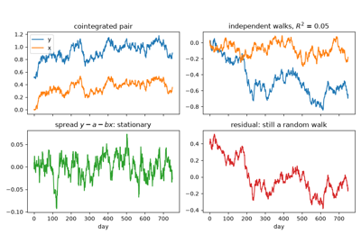
Granger and Newbold (1974) had shown that regressions between independent random walks routinely produce high \(R^2\) and “significant” coefficients. Yet economic theory ties some nonstationary series together, such as consumption and income, spot and futures prices, or a stock’s two share classes. Clive Granger called such series cointegrated: each wanders, but a linear combination does not. Engle and Granger proved that cointegrated series have an error-correction representation and proposed a two-step test. The first step regresses the levels, and the second tests the residuals for a unit root, using critical values that account for the estimated coefficients.

\[y_t = a + b\,x_t + u_t, \qquad u_t \sim I(0) \iff y, x \text{ cointegrated}\]

Implementation: financialkit.time_series.systems.unit_roots.engle_granger() returns a CointegrationResult with MacKinnon’s critical values for two to four variables; simulate_cointegrated_pair() builds test pairs.

References: R. F. Engle and C. W. J. Granger, “Co-Integration and Error Correction: Representation, Estimation, and Testing,” Econometrica 55(2) (1987) 251-276; C. W. J. Granger and P. Newbold, “Spurious Regressions in Econometrics,” Journal of Econometrics 2(2) (1974) 111-120.

Engle-Granger cointegration

1988 – Lo-MacKinlay Variance Ratio #

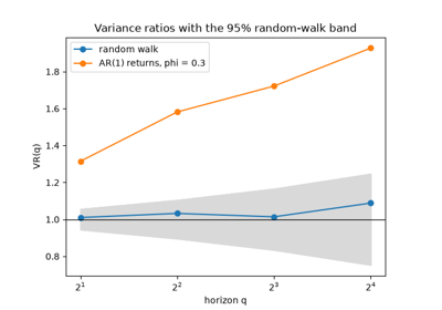
If log prices are a random walk, the variance of \(q\)-period returns grows in proportion to \(q\). Andrew Lo and Craig MacKinlay built a test on the ratio of the two variances. It uses overlapping observations, corrects for bias, and has a standard error that stays valid under volatility clustering. On weekly U.S. stock returns from 1962 to 1985 it rejected the random walk decisively, chiefly through the positive autocorrelation of small-stock portfolios. The paper’s title, “Stock Market Prices Do Not Follow Random Walks,” reopened the debate that Kendall and Fama seemed to have settled.

\[VR(q) = \frac{\hat\sigma^2_c(q)}{\hat\sigma^2_a} \approx 1 + 2\sum_{k=1}^{q-1}\Bigl(1 - \frac kq\Bigr)\rho_k, \qquad z^*(q) = \frac{\sqrt T\,(VR(q) - 1)}{\sqrt{\hat\theta(q)}}\]

Implementation: financialkit.time_series.systems.efficiency.variance_ratio() returns a VarianceRatioResult with both the homoskedastic and the heteroskedasticity-consistent statistics; plot_variance_ratio().

References: A. W. Lo and A. C. MacKinlay, “Stock Market Prices Do Not Follow Random Walks: Evidence from a Simple Specification Test,” Review of Financial Studies 1(1) (1988) 41-66; J. Y. Campbell, A. W. Lo and A. C. MacKinlay, The Econometrics of Financial Markets (Princeton, 1997), Ch. 2.

Lo-MacKinlay variance ratio

1991 – Nelson’s EGARCH #

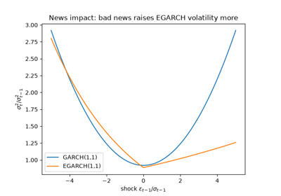
GARCH responds to the size of a shock but not to its sign, and its coefficients need positivity constraints. Daniel Nelson modelled the logarithm of the variance instead. The variance is then positive by construction, and a term in the signed standardized shock lets bad news raise volatility more than good news of the same size. This is the leverage effect that Black (1976) had observed in stock returns. Nelson also worked out the model’s stationarity and moments, and found a strongly negative asymmetry in daily returns on the U.S. stock market.

\[\ln\sigma_t^2 = \omega + \beta\ln\sigma_{t-1}^2 + \alpha\bigl(|z_{t-1}| - E|z|\bigr) + \gamma\,z_{t-1}\]

Implementation: financialkit.time_series.systems.garch.EGARCH, with the closed-form unconditional variance for normal innovations; plot_news_impact() compares news impact curves.

References: D. B. Nelson, “Conditional Heteroskedasticity in Asset Returns: A New Approach,” Econometrica 59(2) (1991) 347-370; F. Black, “Studies of Stock Price Volatility Changes,” Proceedings of the American Statistical Association, Business and Economic Statistics Section (1976) 177-181.

Nelson’s EGARCH

Nelson's EGARCH

1993 – Glosten-Jagannathan-Runkle #

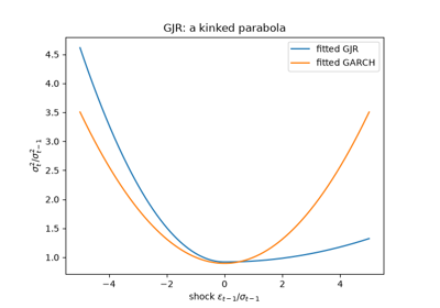
Do investors demand a higher expected return when volatility is high? Estimates of this risk-return trade-off had come out positive, negative or insignificant depending on the volatility model. Lawrence Glosten, Ravi Jagannathan and David Runkle showed that the answer hinged on the asymmetric response of volatility to news. They added a single term to GARCH for negative shocks. On U.S. monthly excess returns nearly all of the response came from bad news. The GJR model keeps GARCH’s analytic forecasts and became, with EGARCH, the standard asymmetric volatility model.

\[\sigma_t^2 = \omega + \bigl(\alpha + \gamma\,\mathbf 1\{\varepsilon_{t-1} < 0\}\bigr)\varepsilon_{t-1}^2 + \beta\,\sigma_{t-1}^2\]

Implementation: financialkit.time_series.systems.garch.GJRGARCH, with persistence \(\alpha + \gamma/2 + \beta\) and analytic forecast().

References: L. R. Glosten, R. Jagannathan and D. E. Runkle, “On the Relation between the Expected Value and the Volatility of the Nominal Excess Return on Stocks,” Journal of Finance 48(5) (1993) 1779-1801.

Glosten-Jagannathan-Runkle

1994 – RiskMetrics EWMA #

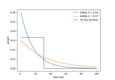
J.P. Morgan’s chairman wanted a single number for the firm’s risk at 4:15 every afternoon. The methodology behind it was published in October 1994, free of charge, as RiskMetrics. Its volatility model was an exponentially weighted moving average of squared returns, with one decay factor for every asset: \(\lambda = 0.94\) for daily data and \(0.97\) for monthly. It is a GARCH(1,1) without a constant and with unit persistence. It needs no estimation and adapts quickly, and it became the industry’s default and the template for Value-at-Risk reporting.

\[\sigma_t^2 = \lambda\,\sigma_{t-1}^2 + (1 - \lambda)\,r_{t-1}^2\]

Implementation: financialkit.time_series.systems.garch.EWMA (lam=0.94 by default; fit() estimates \(\lambda\) by maximum likelihood instead).

References: J.P. Morgan/Reuters, RiskMetrics – Technical Document, 4th ed. (New York, 1996), Ch. 5.

RiskMetrics EWMA

1998 – Andersen-Bollerslev Realized Volatility #

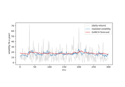
Regressions of squared daily returns on GARCH forecasts gave \(R^2\) of a few percent, and critics concluded that volatility models were useless out of sample. Torben Andersen and Tim Bollerslev showed that the squared return is to blame. It is an unbiased but extremely noisy measure of the day’s variance, so even a perfect forecast explains little of it. Summing squared intraday returns gives realized variance, which converges to the day’s integrated variance. Against it the same forecasts explain far more. Realized measures went on to underpin variance swaps and a new generation of volatility forecasting models.

\[RV_t = \sum_{i=1}^{m} r_{t,i}^2 \;\xrightarrow{\;m\to\infty\;}\; \int_{t-1}^{t}\sigma_s^2\,ds\]

Implementation: financialkit.time_series.systems.realized.realized_variance() and mincer_zarnowitz(); simulate_intraday_returns() spreads each day’s variance over intraday returns.

References: T. G. Andersen and T. Bollerslev, “Answering the Skeptics: Yes, Standard Volatility Models Do Provide Accurate Forecasts,” International Economic Review 39(4) (1998) 885-905; J. Mincer and V. Zarnowitz, “The Evaluation of Economic Forecasts,” in Economic Forecasts and Expectations (New York: NBER, 1969), 3-46.

Andersen-Bollerslev realized volatility