Breakthroughs in Fixed Income#

financialkit.fixed_income hub · History · Examples · API reference

“Gentlemen prefer bonds.” – attributed to Andrew Mellon

A bond promises fixed payments on fixed dates, so its value depends on one thing only: the rates at which those payments are discounted. The history of fixed-income analysis is the story of measuring that dependence more and more precisely. It began with a single number (the duration) and a single rate (the yield). It then moved to a whole curve of rates that can be estimated, bootstrapped and fitted, to portfolios built so that rate changes cannot hurt them, and to swaps that trade one stream of payments for another. This chronology traces the ideas behind financialkit.fixed_income.

1938 – Macaulay Duration #

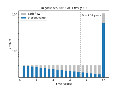
Frederick Macaulay’s NBER study of a century of American interest rates needed a way to compare bonds whose payments are spread over time. Maturity alone ignores the coupons, which return much of the investment before the principal does. Macaulay proposed the present-value-weighted average of the payment times instead. That number is the duration, and it is the balance point of the bond’s discounted cash flows. A zero-coupon bond’s duration equals its maturity, and higher coupons shorten it.

\[D = \frac{1}{P}\sum_i t_i\, c_i\, e^{-y t_i}, \qquad P = \sum_i c_i\, e^{-y t_i}\]

Implementation: financialkit.fixed_income.systems.duration.macaulay_duration(), and bond_risk() for the full BondRisk record.

References: F. R. Macaulay, Some Theoretical Problems Suggested by the Movements of Interest Rates, Bond Yields and Stock Prices in the United States since 1856 (New York: NBER, 1938).

Macaulay duration

1939 – Hicks: Duration as an Elasticity #

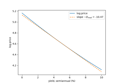
In Value and Capital, John Hicks independently defined the “average period” of a stream of payments. It is the elasticity of the stream’s capital value with respect to the discount factor, and it turns out to be Macaulay’s duration. Read as a sensitivity rather than a time, duration predicts the percentage price change for a small change in yield. In yield units this is modified duration, Macaulay’s number divided by \(1 + y/m\) for a yield compounded \(m\) times a year. Under continuous compounding the two coincide.

\[D_{mod} = -\frac{1}{P}\frac{dP}{dy} = \frac{D_{mac}}{1 + y/m}\]

Implementation: financialkit.fixed_income.systems.duration.modified_duration(), computed from the analytic yield derivatives in yield_discount_derivatives().

References: J. R. Hicks, Value and Capital (Oxford: Clarendon Press, 1939).

Hicks: duration as an elasticity (modified duration)

1940 – Lutz: Forward Rates #

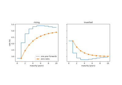
Friedrich Lutz set out the expectations theory of the term structure in a form still taught today. If investors are indifferent between holding a long bond and rolling over short ones, the long rate is an average of expected future short rates. The rates implicit in today’s curve for borrowing over future periods are the forward rates. They lie above the zero curve where it rises and below it where it falls.

\[f(t_1, t_2) = \frac{r(t_2)\, t_2 - r(t_1)\, t_1}{t_2 - t_1}\]

Implementation: financialkit.fixed_income.systems.curves.forward_rates() for a tenor grid, and forward_rate() and instantaneous_forward() on every curve.

References: F. A. Lutz, “The Structure of Interest Rates,” Quarterly Journal of Economics 55(1) (1940), 36-63.

Lutz: forward rates

1952 – Redington Immunization #

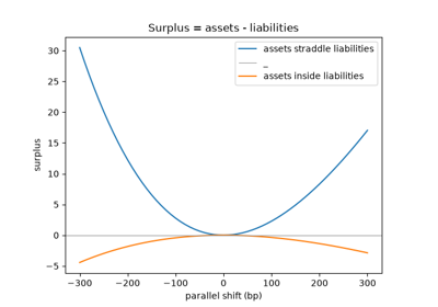
Frank Redington, the Prudential’s actuary, asked how a life office should invest so that a change in interest rates would leave its surplus unharmed. He called the answer immunization. Match the present value of assets to that of liabilities, match their durations, and make the assets’ cash flows more spread out than the liabilities’ (higher convexity). Then any small parallel shift raises the surplus. The surplus as a function of the shift has a minimum at zero.

Implementation: financialkit.fixed_income.systems.immunization.redington_immunize() solves for the two asset holdings and reports the convexity condition in an ImmunizationResult, whose surplus() traces the surplus under parallel shifts.

References: F. M. Redington, “Review of the Principles of Life-Office Valuations,” Journal of the Institute of Actuaries 78(3) (1952), 286-340.

Redington immunization

1971 – Fisher-Weil Duration #

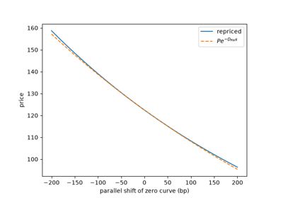
Lawrence Fisher and Roman Weil tested immunization on a century of bond data. They found that it worked, provided the duration was computed with each payment discounted at its own zero rate rather than at the bond’s single yield. Their duration is the exact sensitivity of price to a parallel shift of the zero curve, which is the shift that immunization actually protects against.

\[D_{FW} = \frac{1}{P}\sum_i t_i\, c_i\, e^{-r(t_i)\, t_i} = -\frac{1}{P}\frac{dP}{ds}\]

Implementation: financialkit.fixed_income.systems.duration.fisher_weil_duration() and fisher_weil_convexity(), checked against repricing in effective_duration().

References: L. Fisher and R. L. Weil, “Coping with the Risk of Interest-Rate Fluctuations: Returns to Bondholders from Naive and Optimal Strategies,” Journal of Business 44(4) (1971), 408-431.

Fisher-Weil duration

1971 – McCulloch’s Spline Discount Function #

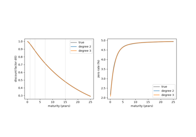
Real bonds do not mature on a neat grid of dates, and their prices are noisy. Huston McCulloch estimated the discount function directly as a spline in maturity. Because a bond’s price is linear in the discount function, it is linear in the spline coefficients too, so the whole curve comes from one least-squares regression on a cross-section of bond prices. His 1971 paper used quadratic splines. The cubic splines of his 1975 paper give smooth forward rates.

Implementation: financialkit.fixed_income.systems.curves.fit_mcculloch_spline() returns a SplineDiscountCurve fitted with numpy.linalg.lstsq().

References: J. H. McCulloch, “Measuring the Term Structure of Interest Rates,” Journal of Business 44(1) (1971), 19-31; J. H. McCulloch, “The Tax-Adjusted Yield Curve,” Journal of Finance 30(3) (1975), 811-830.

McCulloch’s spline discount function

McCulloch's spline discount function

1972 – Inside the Yield Book: Yield to Maturity #

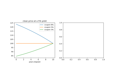
Sidney Homer and Martin Leibowitz of Salomon Brothers wrote the book that made bond mathematics a working tool for traders. Inside the Yield Book explained yield to maturity, the single rate that discounts a bond’s cash flows to its price. It also explained what that yield leaves out, above all the assumption that coupons are reinvested at the same rate. It treated price-yield relations, the pull to par and the value of a basis point as everyday trading arithmetic.

Implementation: financialkit.fixed_income.systems.bonds.yield_to_maturity() inverts price_from_yield() with scipy.optimize.brentq(); accrued_interest() and clean_price() separate the quoted price from the full one.

References: S. Homer and M. L. Leibowitz, Inside the Yield Book: New Tools for Bond Market Strategy (Englewood Cliffs: Prentice-Hall, 1972).

Inside the Yield Book: yield to maturity

1976 – Carleton-Cooper Bootstrapping #

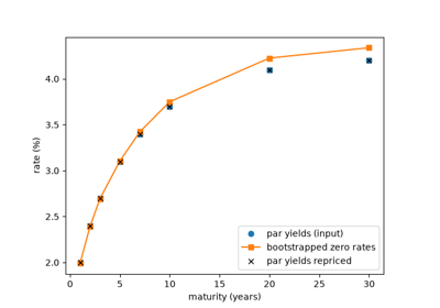
William Carleton and Ian Cooper estimated the term structure from Treasury bonds that pay on common dates. Each price is then a linear combination of the discount factors for those dates. With one bond per date the system is triangular and is solved shortest maturity first, a procedure now called bootstrapping. With more bonds than dates it becomes a regression that averages out pricing errors.

Implementation: financialkit.fixed_income.systems.curves.bootstrap_zero_curve() and bootstrap_par_curve() strip a ZeroCurve, one node per bond, solving each node with scipy.optimize.brentq() so that intermediate coupons are discounted on the interpolated curve. carleton_cooper_discount_factors() solves the overdetermined system by least squares.

References: W. T. Carleton and I. A. Cooper, “Estimation and Uses of the Term Structure of Interest Rates,” Journal of Finance 31(4) (1976), 1067-1083; J. C. Hull, Options, Futures, and Other Derivatives, 9th ed. (Pearson, 2015), Sec. 4.5.

Carleton-Cooper bootstrapping

1981 – The IBM-World Bank Swap #

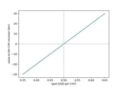
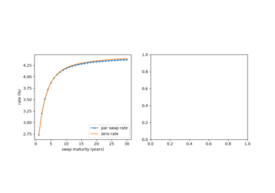
In August 1981 Salomon Brothers arranged for the World Bank to service IBM’s Swiss franc and Deutsche mark debt while IBM serviced dollar debt for the World Bank. Each side obtained the currency it wanted on better terms than it could have borrowed directly. This first widely publicized swap was a fixed-for-fixed currency swap. The single-currency fixed-for-floating interest-rate swap followed in 1982 and became the largest derivatives market in the world. Both kinds are valued as a long position in one bond and a short position in another.

Implementation: financialkit.fixed_income.systems.swaps.currency_swap_value() and interest_rate_swap_value() return a SwapValuation; swap_rate() gives the par swap rate.

References: C. W. Smith, C. W. Smithson and L. M. Wakeman, “The Evolving Market for Swaps,” Midland Corporate Finance Journal 3(4) (1986), 20-32; J. C. Hull, Options, Futures, and Other Derivatives, 9th ed. (Pearson, 2015), Ch. 7.

The IBM-World Bank currency swap

The plain-vanilla interest-rate swap

1983 – Bierwag-Kaufman-Toevs: Convexity #

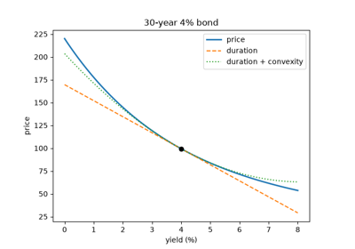
Duration is a tangent to the price-yield curve, and the curve bends. Gerald Bierwag, George Kaufman and Alden Toevs surveyed duration’s development and use in portfolio management, and they made the second-order term, convexity, part of standard practice. With convexity, the price change for a large yield move is predicted far better. A barbell is more convex than a bullet of the same duration, so it gains more when rates move in either direction, as long as the move is a parallel one.

\[\frac{\Delta P}{P} \approx -D_{mod}\,\Delta y + \tfrac12\, C\,(\Delta y)^2, \qquad C = \frac{1}{P}\frac{d^2 P}{dy^2}\]

Implementation: financialkit.fixed_income.systems.duration.convexity() and price_change().

References: G. O. Bierwag, G. G. Kaufman and A. Toevs, “Duration: Its Development and Use in Bond Portfolio Management,” Financial Analysts Journal 39(4) (1983), 15-35.

Bierwag-Kaufman-Toevs: convexity

1984 – Fong-Vasicek M-Squared #

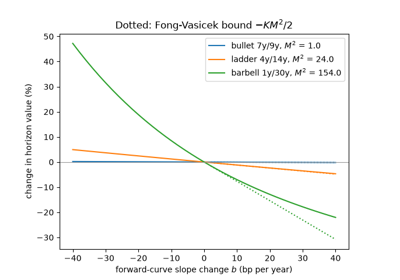
Redington’s conditions guard only against parallel shifts. Gifford Fong and Oldrich Vasicek bounded the loss of a duration-matched portfolio when the forward curve also twists. The bound is proportional to \(M^2\), the present-value-weighted dispersion of the cash flows around the horizon. Among immunized portfolios, the bullet (low \(M^2\)) is the least exposed to twists, which is exactly the reverse of the barbell’s advantage in convexity.

\[\frac{\Delta V_H}{V_H} \ge -\tfrac12 K M^2, \qquad M^2 = \sum_i w_i\,(t_i - H)^2\]

Implementation: financialkit.fixed_income.systems.immunization.m_squared(), fong_vasicek_bound(), horizon_value() and linear_forward_shock().

References: H. G. Fong and O. A. Vasicek, “A Risk Minimizing Strategy for Portfolio Immunization,” Journal of Finance 39(5) (1984), 1541-1546.

Fong-Vasicek M-squared

1985 – STRIPS: a Bond as a Portfolio of Zeros #

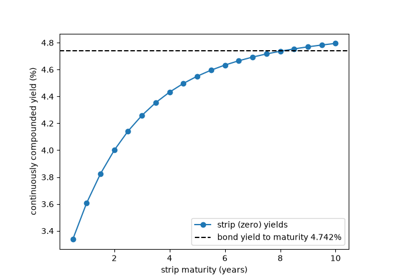
In February 1985 the US Treasury launched STRIPS, the Separate Trading of Registered Interest and Principal of Securities. Dealers could split a note or bond into one zero-coupon security for each payment date, and later reassemble them. This replaced the dealer-created zero receipts of the early 1980s. The idea that a coupon bond is a portfolio of zeros became a traded fact. Stripping and reconstitution keep a bond’s price in line with the zero curve, and STRIPS prices give a zero curve directly.

Implementation: financialkit.fixed_income.systems.bonds.strips_decomposition(), strips_value() and strips_curve().

References: F. J. Fabozzi, Bond Markets, Analysis, and Strategies, 9th ed. (Pearson, 2015), Ch. 6.

STRIPS: a bond as a portfolio of zeros

1987 – Nelson-Siegel #

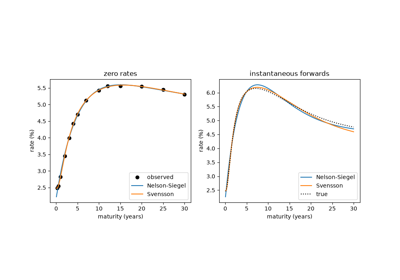
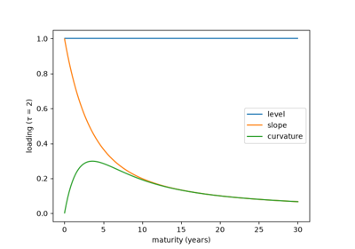
Charles Nelson and Andrew Siegel proposed a parsimonious curve with four parameters: a long-run level, a slope that decays away from the short end, and a hump whose location is set by one decay parameter. It fits the usual shapes of yield curves (rising, inverted, humped) with few parameters. Its parameters later came to be read as the level, slope and curvature factors.

\[r(t) = \beta_0 + \beta_1 \frac{1-e^{-t/\tau}}{t/\tau} + \beta_2\left(\frac{1-e^{-t/\tau}}{t/\tau} - e^{-t/\tau}\right)\]

Implementation: financialkit.fixed_income.systems.curves.NelsonSiegelCurve and fit_nelson_siegel(), which grid-searches \(\tau\) (on which the betas are linear) and refines with scipy.optimize.least_squares().

References: C. R. Nelson and A. F. Siegel, “Parsimonious Modeling of Yield Curves,” Journal of Business 60(4) (1987), 473-489.

Nelson-Siegel

1991 – Litterman-Scheinkman: Level, Slope, Curvature #

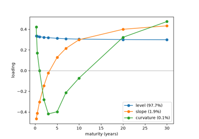
Robert Litterman and José Scheinkman of Goldman Sachs ran a principal component analysis of Treasury returns and found that three factors explain almost all of their variation. They are a near-parallel level shift, a steepness (slope) twist and a curvature bend. Hedging those three factors, rather than duration alone, became standard practice.

Implementation: financialkit.fixed_income.systems.curves.yield_curve_pca() (eigen-decomposition by numpy.linalg.eigh()) returns a CurvePCAResult; simulate_yield_changes() generates factor-driven test data.

References: R. Litterman and J. Scheinkman, “Common Factors Affecting Bond Returns,” Journal of Fixed Income 1(1) (1991), 54-61.

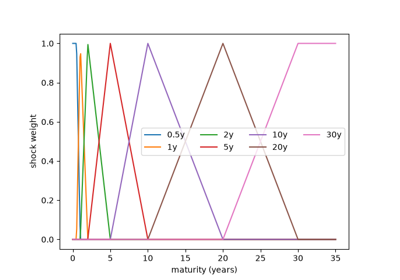
Litterman-Scheinkman: level, slope, curvature

1992 – Ho’s Key Rate Durations #

Thomas Ho replaced the single duration with a vector. Shock one key rate at a time, with triangular shapes that sum to a parallel shift, and measure the price sensitivity to each. The key rate durations add up to the effective duration. They show where along the curve a portfolio’s risk sits, so portfolios with equal durations but different exposures can be told apart and hedged.

Implementation: financialkit.fixed_income.systems.duration.key_rate_durations() returns a KeyRateDurationResult, using the shock shapes of key_rate_weights().

References: T. S. Y. Ho, “Key Rate Durations: Measures of Interest Rate Risks,” Journal of Fixed Income 2(2) (1992), 29-44.

Ho’s key rate durations

Ho's key rate durations

1994 – Svensson #

Lars Svensson, estimating forward rates for the Swedish central bank, added a second hump term with its own decay to Nelson-Siegel. The extra flexibility fits forward curves that bend twice. Many central banks use the Svensson model to estimate and publish their government yield curves.

Implementation: financialkit.fixed_income.systems.curves.SvenssonCurve and fit_svensson().

References: L. E. O. Svensson, “Estimating and Interpreting Forward Interest Rates: Sweden 1992-1994,” NBER Working Paper 4871 (1994).

Svensson