Aliasing before reconstruction

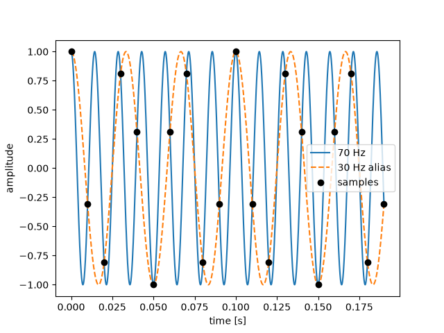
A 70 Hz cosine sampled at 100 Hz is indistinguishable from a 30 Hz cosine. Checking the samples demonstrates why filtering after sampling cannot recover the original frequency.

import matplotlib.pyplot as plt
import numpy as np

from engineeringkit.signal_processing import alias_frequency

fs, frequency = 100, 70
t = np.arange(20) / fs
alias = alias_frequency(frequency, fs)
assert np.isclose(alias, 30)
np.testing.assert_allclose(np.cos(2 * np.pi * frequency * t), np.cos(2 * np.pi * alias * t), atol=1e-13)
fine = np.linspace(0, t[-1], 2001)
fig, ax = plt.subplots()
ax.plot(fine, np.cos(2 * np.pi * frequency * fine), label="70 Hz")
ax.plot(fine, np.cos(2 * np.pi * alias * fine), linestyle="--", label="30 Hz alias")
ax.plot(t, np.cos(2 * np.pi * frequency * t), "ko", label="samples")
ax.set(xlabel="time [s]", ylabel="amplitude")
ax.legend()

plt.show()