
Electrical engineering exercises#
Three problems built on the electrical engineering gallery. Try each one before opening its solution. The solutions run when the documentation is built, and the test suite checks every number they print.
1. Charging a capacitor#
A 100 µF capacitor charges from 12 V through 10 kΩ. How long does it take to reach 90% of the supply voltage? Check the answer \(t = RC\ln 10\) against the charging curve, and find the fraction of the energy drawn from the supply that ends up stored in the capacitor.
Builds on: Examples.
Solution
import numpy as np

from engineeringkit.electrical_engineering import rc_charging_voltage, rc_time_constant

V, R, C = 12.0, 10e3, 100e-6
tau = rc_time_constant(R, C)
t90 = tau * np.log(10)
print(f"tau = {tau:.2f} s, t90 = {t90:.3f} s, v(t90) = {rc_charging_voltage(V, R, C, t90):.3f} V")
# tau = 1.00 s, t90 = 2.303 s, v(t90) = 10.800 V
assert np.isclose(rc_charging_voltage(V, R, C, t90), 0.9 * V)

# The supply delivers charge C V at voltage V; the capacitor stores C V^2 / 2.
stored, drawn = 0.5 * C * V**2, C * V * V
print(f"stored {1e3 * stored:.1f} mJ of {1e3 * drawn:.1f} mJ drawn: {stored / drawn:.0%}")
# stored 7.2 mJ of 14.4 mJ drawn: 50%
Half the energy is always lost in the resistor, whatever its value: a smaller resistor charges faster but dissipates the same energy at a higher power.
2. A series resonant circuit#
A series RLC circuit has \(R = 10\ \Omega\), \(L = 10\) mH and \(C = 1\) µF. Find its resonant frequency, its quality factor \(Q = \sqrt{L/C}/R\), and the impedance at resonance. Find the half-power bandwidth numerically, from the frequencies where \(|Z| = \sqrt2 R\), and compare with \(f_0/Q\).
Builds on: Examples.
Solution
import matplotlib.pyplot as plt
import numpy as np

from engineeringkit.electrical_engineering import SeriesRLC, resonance_frequency, series_rlc_impedance

R, L, C = 10.0, 10e-3, 1e-6
f0 = resonance_frequency(L, C)
Q = np.sqrt(L / C) / R
print(f"f0 = {f0:.1f} Hz, Q = {Q:.1f}, |Z(f0)| = {abs(series_rlc_impedance(R, L, C, 2 * np.pi * f0)):.3f} ohm")
# f0 = 1591.5 Hz, Q = 10.0, |Z(f0)| = 10.000 ohm

f = np.linspace(0.8 * f0, 1.2 * f0, 200_001)
Z = abs(series_rlc_impedance(R, L, C, 2 * np.pi * f))
band = f[Z <= np.sqrt(2) * R]
print(f"half-power band {band[0]:.1f} to {band[-1]:.1f} Hz: width {band[-1] - band[0]:.1f} Hz, f0/Q = {f0 / Q:.1f} Hz")
# half-power band 1514.0 to 1673.1 Hz: width 159.2 Hz, f0/Q = 159.2 Hz
assert np.isclose(band[-1] - band[0], f0 / Q, rtol=1e-4)

result = SeriesRLC(R, L, C).step_response(np.linspace(0, 0.01, 2001))
fig, ax = result.plot()
ax.set_title("1 V step: a lightly damped ring at f0")
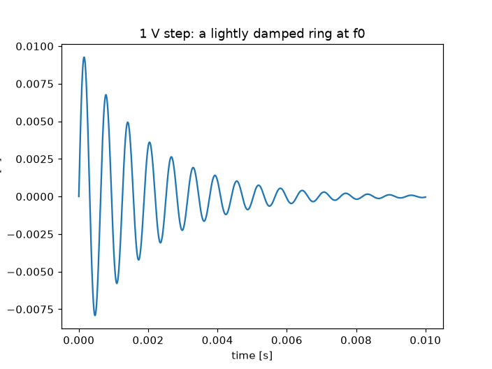
The circuit is lightly damped (\(\zeta = 1/(2Q) = 0.05\)), so its step response rings at the resonant frequency for about \(Q\) cycles.
3. Power-factor correction#
A 230 V, 50 Hz workshop draws 5 kW at a lagging power factor of 0.7. What capacitor in parallel raises the power factor to 0.95, and by how much does it reduce the supply current?
Builds on: Examples.
Solution
import numpy as np

from engineeringkit.electrical_engineering import capacitor_impedance, power_factor, reactive_power, real_power

V, omega, P = 230.0, 2 * np.pi * 50, 5e3
currents = {}
for pf in (0.7, 0.95):
    currents[pf] = P / (V * pf)
    assert np.isclose(real_power(V, currents[pf], pf), P)
Q1 = reactive_power(V, currents[0.7], np.arccos(0.7))
Q2 = reactive_power(V, currents[0.95], np.arccos(0.95))
C = (Q1 - Q2) / (V**2 * omega)
print(f"reactive power {Q1 / 1e3:.2f} kvar -> {Q2 / 1e3:.2f} kvar, capacitor {1e6 * C:.0f} uF")
print(f"supply current {currents[0.7]:.1f} A -> {currents[0.95]:.1f} A")
# reactive power 5.10 kvar -> 1.64 kvar, capacitor 208 uF
# supply current 31.1 A -> 22.9 A
assert np.isclose(V**2 / abs(capacitor_impedance(C, omega)), Q1 - Q2)
assert np.isclose(power_factor(P, np.hypot(P, Q2)), 0.95)
The capacitor supplies the reactive power the motors need locally, so the supply carries 26% less current and the cables and transformer lose 46% less in \(I^2R\).