
Communications exercises#
Three problems built on the communications gallery. Try each one before opening its solution. The solutions run when the documentation is built, and the test suite checks every number they print.
1. Where to put the cable#
A satellite receiver has a low-noise amplifier (gain 30 dB, noise figure 0.8 dB) and a downconverter (gain 20 dB, noise figure 10 dB), joined by a cable with 6 dB of loss. A passive loss at room temperature has a noise figure equal to its loss. Find the system noise figure with the LNA at the dish, before the cable, and with it indoors, after the cable.
Builds on: Friis’s noise formula for cascaded amplifiers.
Solution
import numpy as np

from engineeringkit.communications import cascaded_noise_factor, from_db, noise_figure

lna, cable, converter = (30.0, 0.8), (-6.0, 6.0), (20.0, 10.0)   # (gain dB, NF dB)
for name, chain in (("LNA at the dish", [lna, cable, converter]), ("LNA indoors", [cable, lna, converter])):
    gains, nfs = from_db(np.array(chain).T)
    print(f"{name:15s}: noise figure {noise_figure(cascaded_noise_factor(gains, nfs)):.2f} dB")
# LNA at the dish: noise figure 0.94 dB
# LNA indoors    : noise figure 6.83 dB
assert np.isclose(noise_figure(cascaded_noise_factor(from_db([-6.0, 30.0]), from_db([6.0, 0.8]))), 6.8)
Indoors, the cable’s 6 dB adds directly to the LNA’s noise figure. At the dish, the LNA’s gain makes the cable’s noise negligible. This is why the LNA sits on the antenna.
2. The Shannon limit#
A link receives 1 pW in noise with a density of \(N_0 = 4\times 10^{-21}\) W/Hz. Plot its Shannon capacity against bandwidth from 10 kHz to 10 GHz. Show that the capacity approaches a finite limit, \(P/(N_0 \ln 2)\), and from it find the minimum \(E_b/N_0\) of any reliable link.
Builds on: The Shannon-Hartley capacity of a noisy band-limited channel.
Solution
import matplotlib.pyplot as plt
import numpy as np

from engineeringkit.communications import db, shannon_capacity

P, N0 = 1e-12, 4e-21
B = np.logspace(4, 10, 121)
C = shannon_capacity(B, P / (N0 * B))
limit = P / (N0 * np.log(2))
print(f"capacity at 10 GHz {C[-1] / 1e6:.1f} Mbit/s, limit {limit / 1e6:.1f} Mbit/s")
print(f"minimum Eb/N0 = ln 2 = {db(np.log(2)):.2f} dB")
# capacity at 10 GHz 356.2 Mbit/s, limit 360.7 Mbit/s
# minimum Eb/N0 = ln 2 = -1.59 dB
assert C[-1] < limit and np.isclose(C[-1], limit, rtol=0.02)

fig, ax = plt.subplots(figsize=(5, 3.2))
ax.semilogx(B, C / 1e6, label="capacity")
ax.axhline(limit / 1e6, color="k", ls="--", label="P/(N0 ln 2)")
ax.set(xlabel="bandwidth [Hz]", ylabel="capacity [Mbit/s]")
ax.legend()
fig.tight_layout()
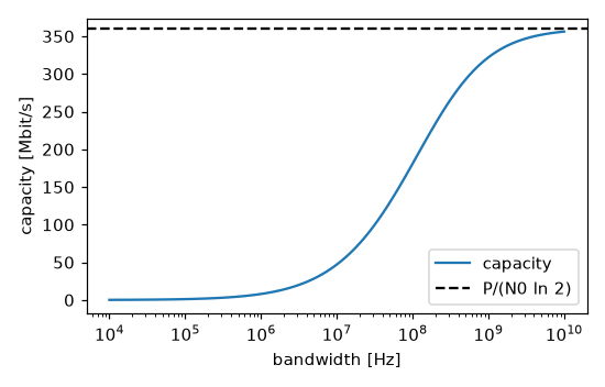
With unlimited bandwidth the bit energy at capacity is \(E_b = P/C = N_0 \ln 2\), so no code can work below \(E_b/N_0 = -1.59\) dB.
3. Carson’s rule and FM broadcasting#
FM broadcast stations use a peak frequency deviation of 75 kHz and audio up to 15 kHz. Estimate the bandwidth with Carson’s rule, compute the modulation index, and compare with the 200 kHz channel spacing.
Builds on: Armstrong’s wideband FM and Carson’s bandwidth rule.
Solution
import numpy as np

from engineeringkit.communications import carson_bandwidth

deviation, audio = 75e3, 15e3
B = carson_bandwidth(deviation, audio)
print(f"modulation index {deviation / audio:.0f}, Carson bandwidth {B / 1e3:.0f} kHz")
# modulation index 5, Carson bandwidth 180 kHz
assert np.isclose(B, 180e3)
180 kHz fits in the 200 kHz channels with a guard band. The modulation index of 5 is what buys FM its noise advantage over AM, at the price of six times the bandwidth.