
Mechanical engineering exercises#
Three problems built on the mechanical engineering gallery. Try each one before opening its solution. The solutions run when the documentation is built, and the test suite checks every number they print.
1. Damping from a free decay#
Damping is hard to calculate but easy to measure: displace the system, let go, and compare successive peaks. Simulate a 1 kg mass on a 4 N/m spring with a 0.4 N s/m damper, released from 0.1 m. Estimate the damping ratio from the logarithmic decrement of the simulated response, and compare it with \(c / (2\sqrt{km})\).
Builds on: Examples.
Solution
import numpy as np

from engineeringkit.mechanical_engineering import damped_frequency, damping_ratio, simulate_sdof

m, c, k = 1.0, 0.4, 4.0
result = simulate_sdof(m, c, k, x0=0.1, t=np.linspace(0, 20, 20001))
x = result.displacement
peaks = np.flatnonzero((x[1:-1] > x[:-2]) & (x[1:-1] > x[2:])) + 1
delta = np.mean(np.log(x[peaks[:-1]] / x[peaks[1:]]))
zeta = delta / np.sqrt(4 * np.pi**2 + delta**2)
period = np.mean(np.diff(result.t[peaks]))
print(f"log decrement {delta:.4f}: zeta {zeta:.4f} (exact {damping_ratio(c, k, m):.4f})")
print(f"damped period {period:.4f} s (exact {2 * np.pi / damped_frequency(k, m, c):.4f} s)")
# log decrement 0.6315: zeta 0.1000 (exact 0.1000)
# damped period 3.1576 s (exact 3.1574 s)
assert np.isclose(zeta, damping_ratio(c, k, m), rtol=1e-3)
The log decrement uses only peak ratios, so it needs no calibration of the displacement sensor’s gain.
2. Isolating a machine#
A 200 kg compressor runs at 1500 rpm. Choose the total stiffness of its rubber mounts (damping ratio 0.05) so that only 10% of its unbalanced force reaches the floor. How far do the mounts deflect under the machine’s weight?
Builds on: Examples.
Solution
import matplotlib.pyplot as plt
import numpy as np
from scipy.optimize import brentq

from engineeringkit.mechanical_engineering import natural_frequency, transmissibility

mass, zeta, omega = 200.0, 0.05, 1500 * 2 * np.pi / 60
r = brentq(lambda r: transmissibility(r, zeta) - 0.1, 1.5, 10)
k = mass * (omega / r) ** 2
print(f"frequency ratio {r:.3f}, stiffness {k / 1e3:.0f} kN/m, static deflection {1e3 * mass * 9.81 / k:.1f} mm")
# frequency ratio 3.399, stiffness 427 kN/m, static deflection 4.6 mm
assert np.isclose(transmissibility(omega / natural_frequency(k, mass), zeta), 0.1)

ratios = np.linspace(0.01, 5, 500)
fig, ax = plt.subplots(figsize=(5, 3.2))
ax.semilogy(ratios, transmissibility(ratios, zeta))
ax.axhline(0.1, color="k", ls=":")
ax.axvline(np.sqrt(2), color="0.6", ls="--")
ax.set(xlabel="frequency ratio r", ylabel="transmissibility")
fig.tight_layout()
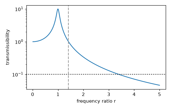
Isolation needs a soft mount: the machine must run at more than \(\sqrt 2\) times the natural frequency, here 3.4 times. Every soft mount has the drawback that the machine passes through resonance as it starts and stops.
3. A gearbox and its bearing#
A motor delivers 10 N m at 1450 rpm into a two-stage gearbox with a 20-tooth pinion driving a 60-tooth gear, then an 18-tooth pinion driving a 54-tooth gear. Each mesh is 98% efficient. Find the output speed and torque. The output shaft’s bearing has a dynamic load rating of 30 kN and carries 4 kN; find its \(L_{10}\) life in hours.
Builds on: Examples.
Solution
import numpy as np

from engineeringkit.mechanical_engineering import bearing_l10_life, gear_output_speed, gear_output_torque, gear_ratio, power_torque

speed, torque = 1450.0, 10.0
for driver, driven in ((20, 60), (18, 54)):
    speed = gear_output_speed(speed, driver, driven)
    torque = gear_output_torque(torque, driver, driven, efficiency=0.98)
print(f"overall ratio {gear_ratio(60, 20) * gear_ratio(54, 18):.0f}: {speed:.1f} rpm, {torque:.1f} N m")
# overall ratio 9: 161.1 rpm, 86.4 N m
power_in = power_torque(10.0, 1450 * 2 * np.pi / 60)
power_out = power_torque(torque, speed * 2 * np.pi / 60)
assert np.isclose(power_out / power_in, 0.98**2)

L10 = bearing_l10_life(30e3, 4e3)
print(f"L10 = {L10:.3e} revolutions = {L10 / (speed * 60):.0f} hours")
# L10 = 4.219e+08 revolutions = 43642 hours
Ball-bearing life goes as the cube of the load ratio: doubling the load cuts the life by eight. The slow output shaft turns few revolutions, so the same bearing lasts nine times longer there than on the motor shaft.