Rayleigh’s Theory of Sound: free vibration (1877)

Lord Rayleigh’s The Theory of Sound (1877) treated every vibrating system, from strings to bells, as a set of linear oscillators. The simplest is a mass on a spring with a dashpot, \(m\ddot x + c\dot x + kx = 0\). It rings at \(\omega_n = \sqrt{k/m}\) (natural_frequency()), and damping lowers the frequency to \(\omega_n\sqrt{1 - \zeta^2}\) (damped_frequency(), damping_ratio()). Rayleigh also showed how to estimate a frequency from energy alone: equate the peak kinetic and potential energies for an assumed shape. With a linear stretch profile, a spring’s own mass \(m_s\) adds \(m_s/3\) to the moving mass. The example checks the simulated response (simulate_sdof()) and Rayleigh’s correction against the exact solution.

import matplotlib.pyplot as plt
import numpy as np
from scipy.optimize import brentq

from engineeringkit.mechanical_engineering import damped_frequency, damping_ratio, natural_frequency, natural_frequency_hz, simulate_sdof

Free decay

Release a 2 kg mass on an 800 N/m spring from 10 mm. Time the peaks of the simulated response and compare with the damped frequency.

m, k = 2.0, 800.0
t = np.linspace(0, 2, 40001)
fig, axes = plt.subplots(1, 2, figsize=(10, 3.8))
for c in (0.0, 4.0, 16.0):
    result = simulate_sdof(m, c, k, x0=0.01, t=t)
    x = result.displacement
    peaks = np.flatnonzero((x[1:-1] > x[:-2]) & (x[1:-1] > x[2:])) + 1
    period = np.mean(np.diff(t[peaks]))
    zeta = damping_ratio(c, k, m)
    print(f"zeta = {zeta:.3f}: measured {2 * np.pi / period:.4f} rad/s, omega_d = {damped_frequency(k, m, c):.4f} rad/s")
    assert np.isclose(2 * np.pi / period, damped_frequency(k, m, c), rtol=1e-4)
    axes[0].plot(t, 1e3 * x, label=f"zeta = {zeta:.2f}")
print(f"undamped: {natural_frequency(k, m):.1f} rad/s = {natural_frequency_hz(k, m):.3f} Hz")
axes[0].set(xlabel="time [s]", ylabel="displacement [mm]", title="Free decay")
axes[0].legend()

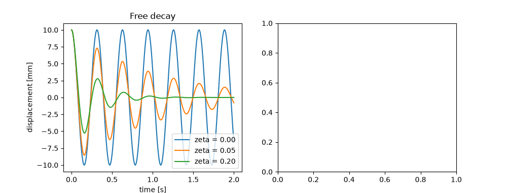
zeta = 0.000: measured 20.0000 rad/s, omega_d = 20.0000 rad/s
zeta = 0.050: measured 19.9752 rad/s, omega_d = 19.9750 rad/s
zeta = 0.200: measured 19.5964 rad/s, omega_d = 19.5959 rad/s
undamped: 20.0 rad/s = 3.183 Hz

<matplotlib.legend.Legend object at 0x111256710>

Rayleigh’s correction for the spring’s mass

A uniform spring fixed at one end and carrying the mass at the other has the exact fundamental \(\omega = \beta\sqrt{k/m_s}\) with \(\beta\tan\beta = m_s/m\). Rayleigh’s energy estimate is \(\sqrt{k/(m + m_s/3)}\).

ratios = np.linspace(0.01, 2, 100)
exact = np.array([brentq(lambda b, s=s: b * np.tan(b) - s, 1e-9, np.pi / 2 - 1e-9) * np.sqrt(k / (s * m)) for s in ratios])
rayleigh = natural_frequency(k, m * (1 + ratios / 3))
naive = natural_frequency(k, m) * np.ones_like(ratios)
error = rayleigh / exact - 1
equal = np.argmin(abs(ratios - 1))
print(f"spring as heavy as the mass: exact {exact[equal]:.3f}, Rayleigh {rayleigh[equal]:.3f} rad/s")
assert np.all(error >= 0) and np.max(error[ratios <= 1]) < 0.01
axes[1].plot(ratios, 100 * error, label="Rayleigh, m + m_s/3")
axes[1].plot(ratios, 100 * (naive / exact - 1), label="spring mass ignored")
axes[1].set(xlabel="spring mass / end mass", ylabel="frequency error [%]", title="Rayleigh's energy estimate")
axes[1].legend()
fig.tight_layout()

plt.show()

spring as heavy as the mass: exact 17.218, Rayleigh 17.331 rad/s